AFQuery
Fast, file-based genomic allele frequency queries for large cohorts. No server, no cloud — just files.
AFQuery stores genotype data as Roaring Bitmaps in Parquet files and answers allele frequency queries in under 100 ms across large cohorts, with flexible filtering by sex, phenotype codes (arbitrary sample labels), and sequencing technology.
When to Use AFQuery
- You need allele frequencies for phenotype-defined subgroups (not just whole-population AF)
- You mix WGS, WES, and panels in one cohort and need technology-aware AN
- You require reproducible local AF computed on your own samples — not just public reference databases
- You run repeated queries on the same dataset (annotation, clinical interpretation, research)
- You need sub-100 ms query latency without database servers or cloud infrastructure
How It Works
AFQuery pre-indexes genotypes as Roaring Bitmaps in Parquet files. At query time, it intersects carrier bitmaps with eligible-sample bitmaps (determined by sex, phenotype, and capture filters) and counts bits — reducing each query to microsecond-scale bitmap operations with sub-100 ms end-to-end latency.
Features
- Sub-100 ms queries — bitmap operations, not VCF scanning. Latency is independent of cohort size.
- Incremental updates — add or remove samples without rebuilding the database.
- Multi-dimensional filtering — filter by sex, phenotype codes, and sequencing technology with include/exclude semantics.
- Server-less — a directory of Parquet files + SQLite. Copy to share, no daemon required.
- Ploidy-aware — correct AN on chrX PAR/non-PAR, chrY, and chrM.
- Technology-aware AN — per-position capture BED intersection across WGS, WES kits, and panels.
- Carrier lookup — list samples carrying any variant with full metadata (sex, tech, phenotypes, genotype, FILTER status).
- VCF annotation — add
AFQUERY_AC/AN/AF/N_HET/N_HOM_ALT/N_HOM_REF/N_FAIL/N_NO_COVERAGEINFO fields from any sample subset. - Audit changelog — every database operation is recorded for reproducibility.
Architecture
graph TD
    A["🔍 Input VCFs<br/>single-sample"]
    B["📥 Ingest<br/>cyvcf2 reads VCFs →<br/>per-sample Parquet files emitted"]
    C["🏗️ Build<br/>DuckDB aggregates per bucket →<br/>Roaring Bitmaps → Parquet"]
    D["💾 Database on Disk<br/>variants/chr*/bucket_*.parquet<br/>capture/*.pkl<br/>metadata.sqlite<br/>manifest.json"]
    E["⚡ Query Engine<br/>Load bitmap → filter samples →<br/>compute AC/AN/AF<br/>~10-100ms"]
    F["📊 Annotate"]
    G["🔄 Update"]

    A --> B
    B --> C
    C --> D
    D --> E
    E -.->|VCF| F
    E -.->|Batch| G
    G -.->|Updated| D

    style A fill:#e1f5ff
    style B fill:#fff3e0
    style C fill:#f3e5f5
    style D fill:#e8f5e9
    style E fill:#fce4ec
    style F fill:#fce4ec
    style G fill:#fce4ec
Where to Start
graph TD
    A["What do you want to do?"]
    B["Build a database<br/>from VCFs"]
    C["Query allele<br/>frequencies"]
    D["Annotate a<br/>patient VCF"]
    E["Classify variants<br/>using ACMG criteria"]
    F["Compare AF across<br/>groups"]

    M["Find carriers of<br/>a variant"]

    A -->|First time| G["5-Min Quickstart"]
    A -->|Build| B
    A -->|Query| C
    A -->|Annotate| D
    A -->|Classify| E
    A -->|Compare| F
    A -->|Carriers| M

    B --> H["Create a Database"]
    C --> I["Query Guide"]
    D --> J["Annotate a VCF"]
    E --> K["ACMG Criteria"]
    F --> L["Cohort Stratification"]
    M --> N["Variant Info"]

    click G "getting-started/quickstart/"
    click H "guides/create-database/"
    click I "guides/query/"
    click J "guides/annotate-vcf/"
    click K "use-cases/acmg-use-cases/"
    click L "use-cases/cohort-stratification/"
    click N "guides/variant-info/"

    style A fill:#e3f2fd
    style G fill:#e8f5e9
Next Steps
- Why Local AF Matters — population gaps, technology bias, and the research behind AFQuery
- Installation — pip, conda, from source
- Quickstart — 5-minute end-to-end tutorial
- Key Concepts — bitmaps, Parquet, manifest, metadata model
Getting Started
Why Local Allele Frequencies Matter
Clinical Decisions Depend on Accurate AF
Allele frequency (AF) is one of the strongest lines of evidence in clinical variant classification. Under the ACMG/AMP framework, AF thresholds directly determine whether a variant is classified as benign (BA1: AF > 5%), supporting-pathogenic (PM2: absent or extremely rare), or strongly pathogenic through case enrichment (PS4). A misestimated AF can flip a classification — and with it, a clinical decision.
Yet AF is not an intrinsic property of a variant — it depends on the population in which it is measured. The same variant can be common in one cohort and absent in another. When the reference population does not match the patient's background, variant classification becomes unreliable.
This page describes four methodological gaps in current allele frequency workflows that AFQuery was designed to address.
Gap 1 — Global Databases Miss Population-Specific Signals
Population databases like gnomAD are invaluable for identifying common variants, but they aggregate data from broad, predominantly European-ancestry populations. When the patient's ancestry differs from the reference, AF estimates diverge — sometimes dramatically.
Real-world impact
Turkish breast cancer variants showed up to 354-fold higher allele frequencies in a local variome compared to gnomAD, leading to 6.7% of VUS being reclassified to likely benign when population-matched data were used (Agaoglu et al., 2024). In Taiwanese inherited retinal degeneration, using a local biobank as ancestry-matched controls for PS4 evidence upgraded 2 variants from LP to P and 6 from VUS to LP (Huang et al., 2026).
The problem extends beyond rare ancestries. In a UK arrhythmia clinic, 32.2% of VUS were reclassified upon re-evaluation with updated frequency data (Young et al., 2024). Analysis of 469,803 UK Biobank exomes found that 12.4% of rare LDLR VUS met criteria for reclassification to likely pathogenic when biobank-derived odds ratios were calibrated to ACMG PS4 strength levels (Bhat et al., 2025).
These are not edge cases. Every cohort with a population composition that differs from gnomAD — geographically, clinically, or by ascertainment — may produce misleading AF when compared only against global references.
| Study | Population | Key Finding |
|---|---|---|
| Agaoglu et al. 2024 | Turkish breast cancer | Up to 354× AF difference vs gnomAD; 6.7% VUS reclassified |
| Huang et al. 2026 | Taiwanese IRD | 8 variants reclassified using local biobank PS4 evidence |
| Young et al. 2024 | UK arrhythmia clinic | 32.2% of VUS reclassified on re-evaluation |
| Bhat et al. 2025 | UK Biobank (470K) | 12.4% rare LDLR VUS reclassifiable via biobank OR |
| Kotan 2022 | Turkish endocrinology | Population-matched variomes correlate best geographically |
| Soussi 2022 | Multi-ethnic (TP53) | 21 benign TP53 SNPs missed in European-biased databases |
| Dawood et al. 2024 | Multi-ethnic (MAVE) | AF evidence codes have inequitable impact on non-Europeans (p = 7.47×10⁻⁶) |
Gap 2 — Mixed Sequencing Technologies Inflate the Denominator
Modern cohorts routinely combine samples sequenced with different technologies — WGS, multiple WES capture kits, and targeted gene panels. Even different versions of the same WES kit can differ by hundreds of base pairs at capture boundaries.
This matters because allele number (AN) must be computed per position, not per cohort. A sample whose capture kit does not cover the queried position has no genotype there: it contributes nothing to AN. If it is naively counted, the denominator is inflated and the resulting AF is artificially deflated.
The figure below illustrates the problem with a minimal example: two versions of the same WES capture kit (V1, n = 120 and V2, n = 80) sequencing a schematic gene with eight exons.
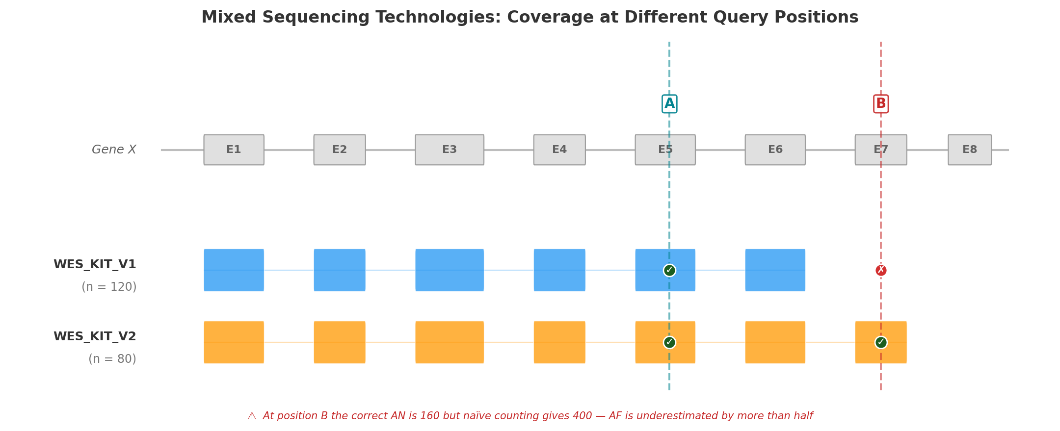
Position A (Exon 5) falls within the capture region of both kit versions. All 200 samples have a genotype at this position, so AN = 200 × 2 = 400. Both kits contribute to the count, and the resulting AF is correct.
Position B (Exon 7) is covered only by WES_KIT_V2. The 120 samples sequenced with V1 have no data at this position. The correct AN is 80 × 2 = 160 — but a naïve calculation that ignores capture boundaries would use 200 × 2 = 400, underestimating AF by more than half. A variant with AC = 5 would appear to have AF = 1.25% (5/400) instead of the true 3.13% (5/160) — enough to cross PM2 filtering thresholds and mislead clinical interpretation.
This is not hypothetical. In the Alzheimer's Disease Sequencing Project, hidden variant-level batch effects between two exome capture kits significantly impacted disease-associated variant identification, with a subset of top risk variants originating exclusively from one kit (Wickland et al., 2021). A population-based WES study found that separating samples by capture protocol yielded 40.9% more high-quality variants than pooling them (Carson et al., 2014).
No general-purpose VCF tool automates per-position, per-technology AN computation across dozens of BED files.
Gap 3 — Static Tools Require Reprocessing
Standard VCF tools — bcftools, VCFtools, GATK — operate on static VCF files. Computing AF over a different sample subset requires:
- Selecting samples by external metadata
- Subsetting the VCF
- Running AF computation
- Repeating for each new subset
This is adequate for one-time analyses but prohibitive for interactive clinical variant interpretation, where a geneticist may need AF across dozens of subsets in a single session: by sex, by phenotype, by technology, by combinations thereof.
For a cohort of 10,000 samples with 5 million variants, reprocessing takes minutes per subset. At 20 subsets per clinical session, the wall time is measured in hours — turning what should be an interactive workflow into a batch job.
Gap 4 — No Metadata-Aware Filtering
Computing AF over "female WGS samples tagged with phenotype E11.9, excluding those also tagged I42" requires orchestrating multiple tools: extract sample IDs from a metadata database, subset the VCF, compute statistics. This multi-step process is error-prone (sample ID mismatches, off-by-one in subsetting) and precludes real-time exploratory analysis.
The lack of integrated metadata filtering is particularly problematic for:
- Pseudo-control analysis — computing AF in all samples except those with a specific disease to assess case enrichment (ACMG PS4)
- Sex-stratified AF — essential for X-linked variant interpretation, where males and females have different ploidy
- Technology-stratified QC — identifying variants that appear only in one sequencing technology, suggesting artifacts rather than true variation
How AFQuery Addresses These Gaps
AFQuery introduces a pre-indexed database architecture that separates the slow step (building the genotype index from VCFs) from the fast step (querying AF on arbitrary subgroups).
The key data structure is the Roaring Bitmap — a compressed bitset that records, for each variant, which samples carry the alternate allele. At query time, computing AC/AN/AF requires only:
- Loading the variant's carrier bitmap from Parquet storage
- Intersecting with the bitmap of eligible samples (determined by sex, phenotype, and capture filters)
- Counting set bits (popcount)
This reduces each query to microsecond-scale bitmap operations, achieving sub-100 ms end-to-end latency including Parquet I/O — regardless of cohort size.
| Gap | Existing tools | AFQuery |
|---|---|---|
| Population-specific AF | Compare against gnomAD; build separate databases per population | Compute AF on any phenotype-defined subgroup at query time |
| Mixed technologies | Manual BED intersection or ignore the problem | Automatic per-position, per-technology AN via capture index |
| Reprocessing | Re-scan VCF per subset (minutes) | Bitmap intersection (milliseconds) |
| Metadata filtering | Multi-step: extract IDs → subset VCF → compute | Single query with --phenotype, --sex, --tech flags |
Next Steps
- Installation — get started
- Key Concepts — how bitmaps, Parquet, and metadata filtering work together
- ACMG Criteria — applying local AF to BA1, PM2, and PS4
Installation
Requirements
- Python 3.10 or later
- For the build phase (
create-db): 2–8 GB RAM per worker (see Performance Tuning)
pip
To install the latest development version directly from GitHub:
conda / mamba (bioconda)
Or with mamba (faster):
Docker
Official images are published to GitHub Container Registry for every release.
Run the CLI by mounting a local directory with your database:
docker run --rm \
  -v /path/to/db:/db \
  ghcr.io/babelomics/afquery:latest \
  query --db /db --locus chr1:925952 --phenotype E11.9
Note
Images are available for linux/amd64 and linux/arm64. The latest tag always points to the most recent stable release.
From Source
To also install documentation dependencies:
Optional: Documentation Dependencies
If you want to build or serve the documentation locally:
Next Steps
- VCF Preprocessing — normalize and prepare VCFs before ingestion
- 5-Min Quickstart — build your first database and run queries
- Key Concepts — understand the bitmap index, manifest, and metadata model
Quickstart
This tutorial walks through building a small AFQuery database and running your first queries. It takes about 5 minutes.
New to AFQuery?
If you want to understand how bitmaps, Parquet storage, and metadata filtering work together before diving in, read Key Concepts first. Otherwise, follow along — you can always come back to the theory later.
Normalize your VCFs first
AFQuery works best with normalized, left-aligned VCFs with ploidy-corrected sex chromosome calls. See VCF Preprocessing for a reference normalization pipeline using bcftools.
1. Create a Manifest
The manifest is a TSV file describing your initial cohort. Create manifest.tsv:
sample_name vcf_path    sex tech_name   phenotype_codes
SAMPLE_001  /data/vcfs/sample001.vcf.gz female  wgs E11.9,I10
SAMPLE_002  /data/vcfs/sample002.vcf.gz male    wgs E11.9
SAMPLE_003  /data/vcfs/sample003.vcf.gz female  wes_v1  I10
Fields:
sample_name: unique identifiervcf_path: path to single-sample VCF (plain or.gz)sex:maleorfemaletech_name: sequencing technology name. UseWGSfor whole genome sequencingphenotype_codes: comma-separated phenotype codes (arbitrary strings)
See Manifest Format for full details.
2. Create the Database
afquery create-db \
  --manifest manifest.tsv \
  --output-dir ./my_db/ \
  --genome-build GRCh38 \
  --bed-dir ./beds/ \
  --threads 12
BED files are required for WES and panel technologies. Place one file per technology in the --bed-dir directory, named <tech_name>.bed (e.g., wes_v1.bed). WGS technologies do not need a BED file.
The command will:
1. Ingest all VCFs
2. Build Roaring Bitmap Parquet files per chromosome/bucket
3. Write manifest.json and metadata.sqlite
3. Inspect the Database (optional)
4. Query a Single Position
Example output:
Filter to female samples with a specific phenotype:
See Sample Filtering for the full include/exclude syntax.
Warnings for missing data
If a phenotype code, technology name, or chromosome is not found in the database, afquery prints a warning to stderr and returns empty results. Use --no-warn to suppress these warnings.
5. Inspect Carriers (optional)
See which samples carry the variant you just queried:
This lists each carrier with their sex, technology, phenotype codes, genotype (het/hom), and FILTER status. See Variant Info for details.
6. Query a Region
7. Annotate a VCF
Given a VCF with variants you want to annotate:
The output VCF gains INFO fields (see Annotate a VCF for parallelism options and downstream usage):
| Field | Number | Description |
|---|---|---|
AFQUERY_AC |
A (per ALT) | Allele count |
AFQUERY_AN |
1 (per site) | Allele number |
AFQUERY_AF |
A (per ALT) | Allele frequency |
AFQUERY_N_HET |
A (per ALT) | Heterozygous sample count |
AFQUERY_N_HOM_ALT |
A (per ALT) | Homozygous alt sample count |
AFQUERY_N_HOM_REF |
A (per ALT) | Homozygous ref sample count |
AFQUERY_N_FAIL |
1 (per site) | Samples with FILTER≠PASS |
AFQUERY_N_NO_COVERAGE |
A (per ALT) | Eligible samples lacking coverage evidence (0 unless a coverage-evidence filter is active) |
Next Steps
- Key Concepts — understand how bitmaps, Parquet, and metadata filtering work together
- Sample Filtering — full syntax for phenotype, sex, and technology filters
- Variant Info — list carriers of any variant with metadata
- Annotate a VCF — annotation options, parallelism, and downstream usage
- ACMG Criteria — applying local AF to BA1, PM2, and PS4
Tutorial: End-to-End Walkthrough
This tutorial walks through every major AFQuery feature using a synthetic demo dataset. By the end, you will have built a database, queried variants, filtered by metadata, annotated a VCF, and exported results.
Prerequisites
Make sure AFQuery is installed. See Installation if needed.
1. Generate Demo Data
AFQuery ships with a script that creates 10 synthetic VCFs, a manifest, and BED files for two WES technologies:
This creates examples/demo/demo_output/ with:
vcfs/— 10 single-sample VCFs (DEMO_001 through DEMO_010)beds/— capture BED files forwes_v1andwes_v2manifest.tsv— sample metadata
The demo cohort has 4 WGS samples, 3 wes_v1 samples, and 3 wes_v2 samples, with phenotype codes E11.9, I10, and control. It includes a set of variants at fixed positions so all query examples in this tutorial produce reproducible output.
2. Create the Database
afquery create-db \
  --manifest examples/demo/demo_output/manifest.tsv \
  --output-dir ./demo_db/ \
  --genome-build GRCh38 \
  --bed-dir examples/demo/demo_output/beds/
This ingests all VCFs, builds Roaring Bitmap Parquet files, and writes manifest.json and metadata.sqlite.
3. Inspect the Database
Example output:
Database:     ./demo_db/
Version:      1.0
Genome build: GRCh38   Schema: 2.0
Created: ...    Updated: N/A

Samples: 10 total
  By sex:       female=5  male=5
  By tech:      wes_v1=3  wes_v2=3  wgs=4
  By phenotype: E11.9=4  I10=5  control=4
The 10 samples span 3 technologies. Phenotype counts reflect samples tagged with each code; a sample may have multiple codes.
4. Query a Single Variant
Query the variant at chr1:925952:
Example output:
Reading the output
Every query result includes the following fields:
| Field | Description |
|---|---|
| AC | Allele count — alt allele copies in eligible samples |
| AN | Allele number — total alleles examined (adjusted for coverage and ploidy) |
| AF | Allele frequency — AC / AN |
| n_eligible | Eligible samples at this position — those passing the metadata filters and covered here. Ploidy is applied afterwards, to AN. Here, 10 = no filter applied and every sample is covered. |
| N_HET | Eligible samples heterozygous for the alt allele |
| N_HOM_ALT | Eligible samples homozygous for the alt allele |
| N_HOM_REF | Eligible samples homozygous reference |
| N_FAIL | Eligible samples with a non-ref allele called but FILTER≠PASS in the source VCF |
For chr1:925952: AN=20 = 10 diploid samples × 2 alleles; AC=6 = 4 het samples (1 copy each) + 1 hom-alt (2 copies).
Accounting identity: n_eligible = N_HET + N_HOM_ALT + N_HOM_REF + N_FAIL + N_NO_COVERAGE always holds. N_NO_COVERAGE is 0 here (it only becomes non-zero with a coverage-evidence filter), so 10 = 4+1+5+0+0 ✓.
N_FAIL in practice
Some variants have samples whose call passed genotyping but failed a quality filter in the source VCF. Query the variant at chr1:946000:
Example output:
Here, 2 samples were flagged as LowQual in their source VCF at this position. N_FAIL samples are:
- Counted in AN — they are eligible and contribute to the denominator
- Excluded from AC — their alleles are not counted in the numerator
This makes AF a conservative estimate: AF=2/20=0.1000 even though 2 additional samples may carry the variant. Verify: 10 = 2+0+6+2 ✓.
Tip
N_FAIL > 0 is a signal to inspect source VCF quality at this site. A high N_FAIL relative to n_eligible may indicate a systematic sequencing artifact. See Understanding Output for thresholds.
Region query
To find all variants in the WES capture region:
Example output:
chr1:925100 C>T  AC=4  AN=20  AF=0.2000  n_eligible=10  N_HET=4  N_HOM_ALT=0  N_HOM_REF=6  N_FAIL=0
chr1:925952 G>A  AC=6  AN=20  AF=0.3000  n_eligible=10  N_HET=4  N_HOM_ALT=1  N_HOM_REF=5  N_FAIL=0
chr1:946000 T>C  AC=2  AN=20  AF=0.1000  n_eligible=10  N_HET=2  N_HOM_ALT=0  N_HOM_REF=6  N_FAIL=2
5. Inspect Variant Carriers
After finding a variant of interest, use variant-info to see which specific samples carry it:
Example output:
sample_id  sample_name  sex     tech    phenotypes       genotype  filter
---------  -----------  ------  ------  ---------------  --------  ------
0          DEMO_001     female  wgs     E11.9,I10        het       PASS
2          DEMO_003     male    wgs     E11.9            het       PASS
4          DEMO_005     female  wes_v1  E11.9,control    het       PASS
6          DEMO_007     male    wes_v2  control          het       PASS
8          DEMO_009     female  wgs     E11.9            hom       PASS
Each row is one carrier. The genotype column shows het (heterozygous), hom (homozygous alt), or alt (non-ref with FILTER≠PASS). The filter column indicates whether the call passed quality filters in the source VCF.
For machine-readable output, use --format tsv:
See Variant Info for full options including allele-specific queries and sample filtering.
6. Filter by Sex
Query only female samples:
Example output:
Now query male samples:
Example output:
AN drops from 20 to 10 in both cases because only 5 samples are eligible. The AF happens to be identical here (0.3000), but the genotype distributions differ: the male group has one homozygous-alt carrier while the female group has three heterozygous carriers.
7. Filter by Phenotype
Query samples tagged with E11.9:
Example output:
Exclude control samples:
Example output:
The ^ prefix means "exclude". Excluding controls removes 4 samples, leaving 6. See Sample Filtering for the full syntax.
8. Filter by Technology
Restrict to WGS samples only:
Example output:
Now query each WES technology separately:
chr1:925952 falls inside the chr1:900000-950000 capture region shared by both WES kits. All 3 wes_v1 samples and all 3 wes_v2 samples are covered, so AN=6 (3 samples × 2 alleles) for both.
The critical case: a position outside all WES capture regions
Now query a position that is not in any WES BED file:
chr1:1399914 lies between the two chr1 WES capture regions (900000–950000 and 1200000–1250000). When you restrict to --tech wes_v1, AFQuery excludes all wes_v1 samples from AN because none of them have coverage at this position — AN=0, so no results are returned.
No variants found ≠ rare
"No variants found" here means AFQuery has no coverage data for the requested technology at this position. The variant exists in the database (visible with --tech wgs), but frequency cannot be estimated for wes_v1. Always check that AN is sufficient before interpreting AF.
9. Combine Filters
All filter dimensions compose with AND:
afquery query \
  --db ./demo_db/ \
  --locus chr1:925952 \
  --sex female \
  --phenotype E11.9 \
  --tech wgs
Example output:
Only one sample meets all three criteria (DEMO_001: female, wgs, E11.9). With n_eligible=1, AN=2 (one diploid sample on an autosome) and AC=1 (heterozygous carrier).
10. Annotate a VCF
Use one of the demo VCFs as input:
afquery annotate \
  --db ./demo_db/ \
  --input examples/demo/demo_output/vcfs/DEMO_001.vcf.gz \
  --output ./annotated_demo.vcf
The output VCF gains AFQUERY_AC, AFQUERY_AN, AFQUERY_AF, AFQUERY_N_HET, AFQUERY_N_HOM_ALT, AFQUERY_N_HOM_REF, and AFQUERY_N_FAIL INFO fields. Inspect the chr1 variants:
Example output (columns: CHROM, POS, ID, REF, ALT, QUAL, FILTER, INFO, FORMAT, DEMO_001):
chr1    925100  .   C   T   50  PASS    AFQUERY_AC=4;AFQUERY_AN=20;AFQUERY_AF=0.2;AFQUERY_N_HET=4;AFQUERY_N_HOM_ALT=0;AFQUERY_N_HOM_REF=6;AFQUERY_N_FAIL=0  GT  0/1
chr1    925952  .   G   A   50  PASS    AFQUERY_AC=6;AFQUERY_AN=20;AFQUERY_AF=0.3;AFQUERY_N_HET=4;AFQUERY_N_HOM_ALT=1;AFQUERY_N_HOM_REF=5;AFQUERY_N_FAIL=0  GT  0/1
chr1    946000  .   T   C   50  PASS    AFQUERY_AC=2;AFQUERY_AN=20;AFQUERY_AF=0.1;AFQUERY_N_HET=2;AFQUERY_N_HOM_ALT=0;AFQUERY_N_HOM_REF=6;AFQUERY_N_FAIL=2  GT  0/1
AFQUERY_N_FAIL=2 for chr1:946000 matches the query output from Step 4. The annotated values reflect cohort-wide frequencies across all 10 samples, not just DEMO_001.
See Annotate a VCF for filtering and downstream usage.
11. Bulk Export with Dump
Export all variant frequencies to CSV:
Preview the first rows:
Example output:
chrom,pos,ref,alt,AC,AN,AF,N_HET,N_HOM_ALT,N_HOM_REF,N_FAIL
chr1,925100,C,T,4,20,0.2,4,0,6,0
chr1,925952,G,A,6,20,0.3,4,1,5,0
chr1,946000,T,C,2,20,0.1,2,0,6,2
chr1,1225000,A,G,5,20,0.25,5,0,5,0
chr1,1399914,G,T,2,8,0.25,2,0,2,0
Note that chr1:1399914 has AN=8 even in the full-cohort dump — technology-aware AN is applied automatically (WES samples are excluded for positions outside their capture regions).
Disaggregate by sex and technology:
This adds columns following the pattern AC_{sex}_{tech}, AN_{sex}_{tech}, AF_{sex}_{tech} (and genotype counts) for each sex-technology combination. The stratified dump is useful for case-control comparisons and population-specific frequency analysis.
12. Interpret Results with ACMG Criteria
With the annotated VCF or query results, you can apply ACMG criteria:
- BA1: Is AF > 5% in your cohort? → Variant is benign.
- PM2_Supporting: Is the variant absent (AC=0) with high AN? → Supporting pathogenic evidence.
- PS4: Is the variant enriched in cases vs. controls? Use
--phenotypeand--phenotype ^disease_codeto compare.
For detailed guidance, see ACMG Criteria (BA1/PM2/PS4).
Next Steps
- Key Concepts — understand how bitmaps, Parquet, and metadata filtering work
- Understanding Output — field definitions and interpretation of N_FAIL, AN=0, and other special cases
- Manifest Format — prepare your own cohort manifest
- Create a Database — build a database from your real data
- ACMG Criteria — apply local AF to variant classification
Key Concepts
Mental Model
AFQuery = bitmap index over genotypes.
For each variant, AFQuery stores a compressed bitset recording which samples carry the alt allele. For each query, it intersects the carrier bitset with an eligible-sample bitset, counts bits, and returns AC/AN/AF.
Samples → Metadata → Filters → Eligible Bitmap
Variants → Genotypes → het/hom Bitmaps
Query: (eligible bitmap) AND (carrier bitmap) → AC; count(eligible) → AN; AC/AN → AF
flowchart LR
    subgraph Input
        S["Samples + Metadata"]
        V["Variants + Genotypes"]
    end

    subgraph Bitmaps
        E["Eligible Bitmap<br/>(sex, phenotype, tech filters)"]
        C["Carrier Bitmap<br/>(het | hom per variant)"]
    end

    subgraph Result
        R["AC = popcount(eligible AND carrier)<br/>AN = popcount(eligible) × ploidy<br/>AF = AC / AN"]
    end

    S --> E
    V --> C
    E --> R
    C --> R

    style E fill:#e3f2fd
    style C fill:#f3e5f5
    style R fill:#e8f5e9
Why Cohort-Specific AF Matters
Allele frequency is not a fixed property of a variant — it is a property of a population. Frequencies vary substantially across ancestry, sequencing technology, and clinical composition. Global databases like gnomAD are invaluable but may not reflect your cohort's background, leading to misestimated AF and incorrect variant classification.
AFQuery lets you compute allele frequencies on exactly the samples in your hands — and on any dynamically defined subset of them — without rebuilding the database.
For a detailed discussion of the methodological gaps AFQuery addresses, including real-world reclassification examples and peer-reviewed references, see Why Local Allele Frequencies Matter.
Allele Frequency (AC / AN / AF)
For a given variant (chromosome, position, ref, alt):
- AC (Allele Count) — number of copies of the alt allele observed across eligible samples
- AN (Allele Number) — total number of alleles examined (2× diploid samples, 1× haploid)
- AF (Allele Frequency) —
AC / AN(None when AN = 0)
A heterozygous carrier contributes AC=1; a homozygous alt carrier contributes AC=2.
Ploidy
AN depends on the chromosome and sex of eligible samples:
| Chromosome | Female | Male |
|---|---|---|
| Autosomes (chr1–22) | 2 | 2 |
| chrX (non-PAR) | 2 | 1 |
| chrX (PAR1/PAR2) | 2 | 2 |
| chrY | 0 | 1 |
| chrM | 1 | 1 |
See Ploidy & Special Chromosomes for PAR coordinates.
Worked Example
Consider a cohort of 60 samples (50 diploid autosomes) with a variant at position chr1:925952 G>A:
| Group | Eligible samples | AN | AC | AF |
|---|---|---|---|---|
| Full cohort (all 60) | 60 samples | 120 | 3 | 0.025 |
| Females only (35) | 35 samples | 70 | 2 | 0.029 |
Tagged E11.9 (20) |
20 samples | 40 | 0 | 0.000 |
Not tagged E11.9 (40) |
40 samples | 80 | 3 | 0.038 |
Tip
AN is not always 2 × cohort_size. Eligible samples change per query, so AN reflects your chosen subgroup exactly.
Visualization
The same variant can show dramatically different allele frequencies across subgroups:
graph TB
    subgraph Full["Full Cohort (60 samples)"]
        F["AC=3, AN=120, AF=0.025"]
    end

    subgraph Females["Females Only (35 samples)"]
        FEM["AC=2, AN=70, AF=0.029"]
    end

    subgraph Disease["Tagged E11.9 (20 samples)"]
        DIS["AC=0, AN=40, AF=0.000"]
    end

    subgraph Controls["Without E11.9 (40 samples)"]
        CTL["AC=3, AN=80, AF=0.038"]
    end

    Full -->|filter| Females
    Full -->|stratify| Disease
    Full -->|exclude| Controls

    style F fill:#e3f2fd
    style FEM fill:#f3e5f5
    style DIS fill:#ffebee
    style CTL fill:#e8f5e9
How AFQuery Stores Data
Per-Variant Bitmaps
For each variant row, AFQuery stores per-sample genotype information as Roaring Bitmaps. Three of them drive every query:
het_bitmap— sample is heterozygous (GT=0/1) withFILTER=PASShom_bitmap— sample is homozygous alt (GT=1/1, orGT=1on haploid regions) withFILTER=PASSfail_bitmap— the sample's call at this site hasFILTER≠PASS
Each sample has a stable integer ID (0-indexed). The bit position in the bitmap equals the sample ID. Databases built with coverage-quality filters carry two additional bitmaps — see Data Model.
Parquet Storage
Bitmaps are serialized and stored in Parquet files, partitioned by chromosome and 1-Mbp bucket:
variants/
  chr1/
    bucket_0.parquet   ← positions 0–999,999
    bucket_1.parquet   ← positions 1,000,000–1,999,999
    ...
  chr2/
    ...
Rows within each bucket are sorted by (pos, alt).
Capture Index (WES)
For whole-exome sequencing (WES) and gene panels technologies, a BED file defines covered regions. AFQuery builds an interval tree (pickle file) per technology so queries can determine which WES samples are eligible at any given position.
WGS samples are always eligible (no BED file needed).
The Manifest
The manifest is a TSV file that drives database creation. It maps each sample to its:
- VCF file path
- Sex (
male/female) - Sequencing technology
- Phenotype codes (arbitrary strings, comma-separated)
The manifest is parsed into metadata.sqlite during create-db. The original path is recorded in manifest.json.
Sample Filtering Model
Queries can restrict the eligible sample set along three independent dimensions:
| Dimension | Filter | Default |
|---|---|---|
| Sex | male, female, or both |
both |
| Phenotype | Include/exclude phenotype codes (arbitrary strings) | all samples |
| Technology | Include/exclude tech names | all samples |
Filters compose with AND across dimensions: a sample must satisfy all three to be eligible.
Within a dimension, multiple include codes compose with OR (a sample matching any code is included).
AN is computed only over eligible samples, so AF naturally reflects the chosen subgroup.
The Metadata Model
AFQuery treats phenotype codes as arbitrary string labels. You can use:
- ICD-10 disease codes (International Classification of Diseases, 10th revision) — e.g.,
E11.9,G40 - Human Phenotype Ontology (HPO) terms — e.g.,
HP:0001250 - OMIM entries (Online Catalog of Human Genes and Genetic Disorders) — e.g.,
OMIM:143100 - Custom project tags (
control,rare_disease,pilot_cohort) - Technology subgroups (
panel_v1,panel_v2) - Any combination of the above
Multiple labels per sample are supported. There is no validation or controlled vocabulary — you define the ontology for your cohort.
When planning phenotype codes, consider:
- Codes can be updated after ingestion using
afquery update-db --update-sample(see Updating sample metadata) - Codes are case-sensitive:
E11.9≠e11.9 - Trailing or leading spaces cause silent mismatch (always use
E11.9,I10, neverE11.9, I10)
PASS-only ingestion is always enforced. See FILTER=PASS Tracking for details.
Next Steps
- 5-Min Quickstart — build your first database and run queries
- Sample Filtering — phenotype, sex, and technology filter syntax
- Ploidy & Special Chromosomes — PAR regions and ploidy rules in detail
VCF Preprocessing
AFQuery ingests single-sample, normalized VCF files. While AFQuery itself does not perform VCF normalization, the accuracy of your allele frequency estimates depends on the quality and consistency of your input VCFs. This page explains why normalization matters and provides a reference pipeline.
A ready-to-use normalization script is provided at resources/normalize_vcf.sh.
Why Normalize?
Left-alignment and decomposition
Multi-allelic variants and complex indels can be represented in multiple equivalent ways in VCF format. Without normalization:
- The same deletion may appear as different ALT alleles depending on the caller
- Multi-allelic sites may not be decomposed into biallelic records
- Duplicate records can inflate AC
bcftools norm left-aligns indels against the reference genome and decomposes multi-allelic sites, ensuring consistent representation across samples.
Ploidy correction for sex chromosomes
Male samples should have haploid genotype calls at chrX non-PAR regions (GT=1, not GT=0/1 or 1/1). Many variant callers output diploid genotypes for males at chrX by default. Without ploidy correction:
- Males at chrX are counted as diploid → AN is inflated by up to 50%
- AF estimates for X-linked variants are systematically underestimated
bcftools +fixploidy corrects genotype ploidy based on a sex file.
Filtering and stripping
- Non-PASS genotypes: Masking them as missing ensures that low-quality calls do not inflate AC. AFQuery tracks these as N_FAIL.
- Homozygous reference calls: Removing ref/ref genotypes reduces file size and speeds ingestion; they contribute AC=0 and are not needed
- INFO fields: Stripping INFO reduces file size and speeds ingestion. Additionally, malformed or non-standard INFO fields produced by some variant callers can break downstream parsing; stripping them pre-emptively prevents these errors.
- FORMAT fields: Only
GT,DP, andGQare preserved.GTis the genotype required by AFQuery for all queries.DPandGQare read by the coverage-evidence quality flags (afquery create-db --min-dp / --min-gq / --min-qual / --min-covered). VCFs withoutDP/GQare still valid; their carriers simply contribute no quality evidence to the cohort. All other FORMAT fields (PL,AD, etc.) are dropped to reduce file size.
Next Steps
- Manifest Format — describe your cohort samples for ingestion
- Create a Database — build the AFQuery database from normalized VCFs
- 5-Min Quickstart — end-to-end tutorial from manifest to first query
Understanding Output
This page explains what each field in AFQuery output means and how to interpret special cases.
Output Fields
| Field | Type | Description |
|---|---|---|
| AC | int | Allele count — number of alt allele copies in eligible samples |
| AN | int | Allele number — total alleles examined (adjusted for ploidy and eligible samples) |
| AF | float | Allele frequency — AC / AN. None when AN=0 |
| N_HET | int | Number of eligible samples heterozygous for the alt allele (GT=0/1) |
| N_HOM_ALT | int | Number of eligible samples homozygous for the alt allele (GT=1/1 or GT=1). Includes haploid carriers on sex chromosomes and chrM. See Ploidy. |
| N_HOM_REF | int | Number of eligible samples homozygous reference (GT=0/0 or GT=0) |
| n_eligible | int | Number of eligible samples — those passing the sex/phenotype/tech filters and covered at this position |
| N_FAIL | int | Number of eligible samples whose call at this position had FILTER≠PASS. These samples are counted only in N_FAIL — not in N_HET, N_HOM_ALT, or N_HOM_REF — but they stay eligible and still count toward AN. |
| N_NO_COVERAGE | int | Number of eligible samples whose tech lacks coverage evidence at this position. Excluded from N_HOM_REF to keep AC/AN conservative. Always 0 unless a coverage-evidence filter is active. See Coverage Evidence. |
Output Formats
Text (default)
chr1:925952 G>A AC=3 AN=120 AF=0.0250 n_eligible=60 N_HET=1 N_HOM_ALT=1 N_HOM_REF=57 N_FAIL=0 N_NO_COVERAGE=0
TSV
chrom   pos ref alt AC  AN  AF  n_eligible  N_HET   N_HOM_ALT   N_HOM_REF   N_FAIL  N_NO_COVERAGE
chr1    925952  G   A   3   120 0.025000    60  1   1   57  0   0
JSON
{
  "chrom": "chr1",
  "pos": 925952,
  "ref": "G",
  "alt": "A",
  "AC": 3,
  "AN": 120,
  "AF": 0.025,
  "n_eligible": 60,
  "N_HET": 1,
  "N_HOM_ALT": 1,
  "N_HOM_REF": 57,
  "N_FAIL": 0,
  "N_NO_COVERAGE": 0
}
Special Cases
AN=0 and AF=None
AN=0 means no eligible samples have coverage at this position. This happens when:
- All eligible samples are WES or panels and the position is outside capture regions
- The phenotype/sex/technology filter excludes all samples
- The chromosome is not in the database
AN=0 does not mean the variant is absent
AN=0 means AFQuery has no data to compute frequency. It is not evidence of rarity.
Warnings
afquery emits a AfqueryWarning to stderr when a query may silently return fewer or no results. Common causes:
| Situation | Warning message |
|---|---|
| Chromosome not in database | Chromosome 'chrXX' has no data in this database. Available: [...] |
| Unknown phenotype code (include) | Phenotype 'CODE' not in database — include will match 0 samples. |
| Unknown phenotype code (exclude) | Phenotype 'CODE' not in database — exclude has no effect. |
| Unknown technology name (include) | Technology 'NAME' not in database — include will match 0 samples. |
| Unknown technology name (exclude) | Technology 'NAME' not in database — exclude has no effect. |
| Contradictory filters (e.g. include + exclude same code) | Sample filter produces an empty eligible set — all queries will return AN=0. |
Use --no-warn to suppress these warnings:
afquery query --db ./my_db/ --locus chr22:1000 --no-warn
afquery annotate --db ./my_db/ --input in.vcf --output out.vcf --no-warn
AC=0 with High AN
AC=0 with a high AN (e.g., AN=4000) means the variant was genuinely not observed in a well-covered cohort. This is meaningful evidence that the variant is rare or absent in your population.
N_FAIL > 0
When N_FAIL > 0, some eligible samples had a non-PASS filter at this position in their source VCF. A high N_FAIL relative to AN may indicate a problematic site (e.g., systematic sequencing artifacts). Consider filtering positions with more than 10% of failing (N_FAIL / (AN / 2) > 0.1).
VCF Annotation Fields
When using afquery annotate, the following INFO fields are added to each variant:
| INFO field | Number | Description |
|---|---|---|
AFQUERY_AC |
A (per ALT) | Allele count — one value per ALT allele |
AFQUERY_AN |
1 (per site) | Allele number — shared across all ALT alleles |
AFQUERY_AF |
A (per ALT) | Allele frequency — one value per ALT allele |
AFQUERY_N_HET |
A (per ALT) | Heterozygous sample count per ALT allele |
AFQUERY_N_HOM_ALT |
A (per ALT) | Homozygous alt sample count per ALT allele |
AFQUERY_N_HOM_REF |
A (per ALT) | Homozygous ref sample count per ALT allele |
AFQUERY_N_FAIL |
1 (per site) | Fail sample count — shared across all ALT alleles |
AFQUERY_N_NO_COVERAGE |
A (per ALT) | Eligible samples whose tech lacks coverage evidence at this position. Always 0 unless a coverage-evidence filter is active. See Coverage Evidence. |
Multi-allelic sites
Number=A fields have one value per ALT allele (comma-separated for multi-allelic sites). Number=1 fields are shared across all ALT alleles at the same position.
These fields can be used directly in downstream filtering with bcftools filter:
# Keep variants rare in cohort with sufficient coverage
bcftools filter -i 'AFQUERY_AF < 0.001 && AFQUERY_AN >= 1000' annotated.vcf.gz
Next Steps
- Key Concepts — how AC, AN, and AF are computed
- Sample Filtering Guide — phenotype, sex, and technology filters
- Annotate a VCF — add AFQUERY_AF/AC/AN fields to a patient VCF
- Clinical ACMG Use Cases — applying local AF to ACMG BS1/PM2 criteria
User Guides
🧬 Bioinformatics Workflows
Create a Database
afquery create-db builds the AFQuery database from a manifest of single-sample VCFs. This is a one-time setup step; incremental updates use afquery update-db.
Basic Usage
For cohorts with WES/panel samples, provide the BED file directory:
afquery create-db \
  --manifest manifest.tsv \
  --output-dir ./db/ \
--genome-build GRCh38 \
--bed-dir ./beds/
What Happens
- Ingest phase — Each VCF is parsed with cyvcf2. Genotypes and quality fields are written to a temporary per-sample Parquet file, one row per variant per sample.
- Build phase — DuckDB reads the temporary Parquet files, aggregates per 1-Mbp bucket, and writes Roaring Bitmap Parquet files partitioned by chromosome and bucket.
- Finalize —
manifest.jsonandmetadata.sqliteare written to the output directory.
Directory Layout After Creation
./db/
├── manifest.json          # Build configuration (genome build, schema version, etc.)
├── metadata.sqlite        # Sample/phenotype/technology/changelog metadata
├── variants/              # Parquet files partitioned by chromosome and bucket
│   ├── chr1/
│   │   ├── bucket_0.parquet      # Positions 0–999,999
│   │   ├── bucket_1.parquet      # Positions 1,000,000–1,999,999
│   │   └── ...
│   ├── chr2/
│   └── ...
└── capture/               # Interval trees for WES technologies (pickle files)
    ├── wes_v1.pkl
    └── wes_v2.pkl
Memory and Thread Tuning
For large cohorts, tune these options:
afquery create-db \
  --manifest manifest.tsv \
  --output-dir ./db/ \
  --genome-build GRCh38 \
  --build-threads 32 \
  --build-memory 4GB
| Option | Default | Recommendation |
|---|---|---|
--build-threads |
all CPUs | Set to min(cpu_count, available_RAM_GB / 2) |
--build-memory |
2GB |
Increase for dense WGS regions or large cohorts |
--threads |
all CPUs | Controls ingest parallelism (VCF parsing) |
The build phase uses one DuckDB process per 1-Mbp bucket. With --build-threads 32 and --build-memory 4GB, peak RAM usage is approximately 32 × 4 = 128 GB.
Resume Behavior
If create-db is interrupted, it resumes automatically from where it left off. Individual bucket Parquet files that were already written are skipped.
To force a complete restart:
Warning
--force deletes all existing output in --output-dir. Use with caution.
FILTER=PASS Behavior
Only FILTER=PASS calls (or calls with no FILTER field) contribute to AC, and therefore to AF. AN is not affected — it counts every eligible sample, failed calls included. Calls that fail a filter are tracked in fail_bitmap and surfaced as N_FAIL. PASS-only counting is always enforced — there is currently no CLI option to change this behaviour.
See FILTER=PASS Tracking for details.
Coverage-Evidence Filters
Four optional flags enable per-sample, quality-aware tracking of which positions each partially-covered technology (WES, panels) actually covered. They are fully opt-in.
| Flag | Default | Effect |
|---|---|---|
--min-dp D |
0 | Minimum FORMAT/DP for a carrier to count as quality evidence. |
--min-gq G |
0 | Minimum FORMAT/GQ for a carrier to count as quality evidence. |
--min-qual Q |
0.0 | Minimum VCF QUAL field for a carrier to count as quality evidence. |
--min-covered K |
0 | Per partially-covered tech, the position is "trusted" only if at least K of its carriers pass the quality thresholds. Non-carriers of failing positions are recorded as N_NO_COVERAGE. |
When any of these flags is non-zero AFQuery reads FORMAT/DP, FORMAT/GQ,
and QUAL from each variant call during ingest. Use the bundled
resources/normalize_vcf.sh (which preserves these FORMAT fields) or ensure
your own preprocessing keeps them.
Example:
afquery create-db \
  --manifest samples.tsv \
  --output-dir ./db/ \
  --genome-build GRCh38 \
  --bed-dir ./beds/ \
  --min-dp 30 --min-gq 20 --min-covered 1
Thresholds are fixed at creation time. update-db --add-samples reuses them
and re-applies them to every position whose partially-covered tech receives
new samples (see Update Database).
See Coverage Evidence for when to reach
for each flag, how N_NO_COVERAGE is computed, and the query-time companion
flag --min-quality-evidence.
Validating the Result
After creation, run:
And inspect database metadata:
Example info output:
Database:       ./db/
Schema version: 2.0
Genome build:   GRCh38
DB version:     1.0
Samples:        1371
Technologies:   wgs, wes_v1, wes_v2
Chromosomes:    chr1 ... chrX chrY chrM
These commands are available at any time after database creation — not only immediately after create-db. Use afquery check to verify database integrity (manifest consistency, Parquet file health, capture index presence) and afquery info to inspect sample counts, registered technologies, and phenotype codes.
Full Option Reference
See CLI Reference → create-db.
Next Steps
- Manifest Format — TSV manifest column reference and common mistakes
- Query Allele Frequencies — run your first queries against the new database
- Performance Tuning — build thread and memory configuration for large cohorts
Manifest Format
The manifest is a tab-separated (TSV) file that describes your sample cohort. It is the primary input to afquery create-db and afquery update-db --add-samples.
Column Specification
| Column | Required | Type | Description |
|---|---|---|---|
sample_name |
Yes | string | Unique identifier for the sample. Must be unique across the entire database. |
vcf_path |
Yes | string | Absolute or relative path to the single-sample VCF file (plain or .gz). |
sex |
Yes | male | female |
Biological sex. Used for ploidy-aware AN computation on sex chromosomes. |
tech_name |
Yes | string | Sequencing technology name (e.g., wgs, wes_v1, capture_kit_A). Case-sensitive. |
phenotype_codes |
No | string | Comma-separated phenotype codes for this sample (arbitrary strings, e.g., E11.9,control). |
Example
sample_name vcf_path    sex tech_name   phenotype_codes
SAMP_001    /data/vcfs/SAMP_001.vcf.gz  female  wgs E11.9,I10
SAMP_002    /data/vcfs/SAMP_002.vcf.gz  male    wgs E11.9
SAMP_003    /data/vcfs/SAMP_003.vcf.gz  female  wes_v1  I10
SAMP_004    /data/vcfs/SAMP_004.vcf.gz  male    wes_v1
SAMP_005    /data/vcfs/SAMP_005.vcf.gz  female  wgs E11.9,I10,N18.3
Header row required
The first row must be the header with exactly these column names.
Phenotype Codes
Naming map
The manifest column is phenotype_codes (plural, comma-separated). The CLI flag is --phenotype (singular, repeatable). In documentation text, "phenotype codes" refers to the values stored in this field.
The phenotype_codes column accepts any arbitrary strings — there is no required ontology. Common choices include:
- ICD-10 disease codes (e.g.,
E11.9,I10,N18.3) - HPO phenotype terms (e.g.,
HP:0001250) - Custom project tags (e.g.,
control,pilot,high_coverage_wgs) - Population or batch labels (e.g.,
EUR,batch_2023) - Technology subgroups (e.g.,
panel_v1,panel_v2)
Multiple codes per sample can be provided (comma-separated, no spaces)
Samples with no phenotype can leave the phenotype_codes column empty
Important
phenotype_codes are stored as-is and matched exactly in queries (case-sensitive)
Technology Names
- Technology names are arbitrary strings — use whatever is meaningful for your cohort
- Common conventions:
wgs,wes_v1,wes_v2,capture_twist_v2
WGS is case-insensitive
The technology name WGS is matched case-insensitively: wgs, WGS, Wgs are all recognized as whole-genome sequencing (no BED file required). All other technology names are case-sensitive and must match exactly between the manifest and the --tech query filter.
- WGS technologies (no BED file): all positions are always eligible
- WES technologies (with BED file): coverage is determined by
<tech>.bedin--bed-dir
WES BED files
For any technology that is not WGS, you must provide a BED file named <tech>.bed in
the --bed-dir directory. If the file is not found, AFQuery aborts with an error before
any ingestion begins:
To resolve this, either supply the correct BED file or rename the technology to WGS
in the manifest (no BED file required for WGS).
BED File Format
BED files for WES capture regions must be:
- 0-based, half-open coordinates (standard BED format)
- Tab-separated with at least 3 columns:
chrom,start,end - Chromosome names matching your VCF style (
chr1or1) - Named
<tech_name>.bed(exact match to thetech_namecolumn in the manifest)
Common Mistakes
| Mistake | Effect | Fix |
|---|---|---|
| Spaces instead of tabs | Parse error | Use \t (Tab key) as separator |
Duplicate sample_name |
Ingest error | Each sample must have a unique name |
| Wrong sex value | Silent error (no ploidy adjustment) | Use exactly male or female |
Spaces in phenotype (E11.9, I10) |
Code " I10" stored with leading space |
Use E11.9,I10 (no spaces) |
| Relative VCF path from wrong CWD | File not found error | Use absolute paths or run from the correct directory |
Next Steps
- Create a Database — use the manifest to build the AFQuery database
- Key Concepts — phenotype code model and metadata filtering
- Sample Filtering — how phenotype codes translate to query filters
Update a Database
afquery update-db adds new samples, removes existing samples, updates sample metadata, and compacts the database to reclaim space.
Update Timeline
graph TD
    A["Initial Build<br/>1000 samples<br/>DB v1.0"]
    B["Add Batch 2<br/>+500 samples<br/>DB v1.1"]
    C["Add Batch 3<br/>+300 samples<br/>DB v1.2"]
    D["Remove<br/>50 samples<br/>DB v1.3"]
    E["Compact<br/>reclaim 2% disk<br/>DB v1.3c"]

    A -->|--add-samples batch2.tsv| B
    B -->|--add-samples batch3.tsv| C
    C -->|--remove-samples SAMP_*| D
    D -->|--compact| E

    style A fill:#e3f2fd
    style B fill:#fff3e0
    style C fill:#fff3e0
    style D fill:#ffebee
    style E fill:#e8f5e9
Add Samples
Provide a new manifest TSV with the samples to add:
The new manifest follows the same format as the original (see Manifest Format). New samples are assigned monotonically increasing sample IDs.
To add multiple manifests at once:
For WES samples, provide the BED file directory:
Coverage-evidence handling
If the database was created with --min-dp / --min-gq / --min-qual /
--min-covered, the existing thresholds are read from the database and
re-applied to all samples — old and new. There is no update-db flag to
override them; thresholds are fixed at creation time so that quality
decisions are comparable across batches.
When new carriers push a partially-covered tech above the --min-covered
threshold at positions that were previously below it, those positions are
re-evaluated and their non-carrier samples once again count as N_HOM_REF
instead of N_NO_COVERAGE. The recomputation runs only for chromosomes
touched by the new samples; existing rows on other chromosomes are not
rewritten.
VCFs added via update-db should preserve FORMAT/DP and FORMAT/GQ (the
bundled resources/normalize_vcf.sh does so by default). Samples without
those fields are still merged correctly but contribute no quality evidence.
See Coverage Evidence for the full flag reference and when to use each one.
Remove Samples
Remove one or more samples by name:
Remove multiple samples:
Or repeat the flag:
Note
Removal marks the sample as inactive and clears its bit from all bitmaps. The physical bit position is not reused. Run --compact after removing many samples to reclaim disk space.
Compact
After removing samples, compact the database to remove dead bits and reduce disk usage:
This rewrites all Parquet files, removing bits for deleted samples. For large databases, compact runs in parallel and may take several minutes.
When to Compact
- After removing more than 5–10% of samples
- When disk space is a concern
- Before archiving or sharing the database
Combine Operations
Operations can be combined in a single command:
afquery update-db \
  --db ./db/ \
  --remove-samples SAMP_OLD_001 \
  --add-samples new_cohort.tsv \
  --compact
Operations execute in this order: remove → add → compact.
Database Version
By default, the version label auto-increments (e.g., 1.0 → 2.0). Set a custom version:
View Changelog
Every update operation is logged. View the history:
Example output:
v1.0  2026-01-15  create   1371 samples added
v2.0  2026-02-01  add       42 samples added
v2.0  2026-02-15  remove     3 samples removed
v3.0  2026-03-01  compact   compacted after removal
Update Sample Metadata
Correct a sample's sex or phenotype_codes without re-ingesting its VCF. Precomputed bitmaps are regenerated and the change is logged in the changelog.
Single sample
# Change sex
afquery update-db --db ./db/ --update-sample SAMP_001 --set-sex female

# Replace phenotype codes (replaces ALL current codes)
afquery update-db --db ./db/ --update-sample SAMP_001 --set-phenotype "E11.9,I10"

# Change both fields in one command
afquery update-db --db ./db/ \
  --update-sample SAMP_001 \
  --set-sex female \
  --set-phenotype "E11.9,I10"
Batch update from TSV
Create a TSV file with a sample_name, field, new_value header. One change per row; the same sample can appear on multiple rows:
sample_name field   new_value
SAMP_001    sex female
SAMP_002    phenotype_codes E11.9,I10
SAMP_003    sex male
SAMP_003    phenotype_codes C50
Operator note
Attach a free-text note to every changelog entry created by the update:
afquery update-db --db ./db/ \
  --update-sample SAMP_001 \
  --set-phenotype "E11.9" \
  --operator-note "Corrected after clinical review 2026-03-19"
Verify the change
# Inspect the changelog
afquery info --db ./db/ --changelog

# List samples to confirm new values
afquery info --db ./db/ --samples

# Query with the updated phenotype
afquery query --db ./db/ --locus chr1:925952 --phenotype E11.9
Full Option Reference
See CLI Reference → update-db.
Next Steps
- Create a Database — initial database creation from a manifest
- Performance Tuning — thread and memory configuration for the build phase
- Multi-cohort Strategies — organizing and versioning databases across cohorts
Query Allele Frequencies
afquery query retrieves allele frequencies from the database. Three query modes are available: point, region, and batch.
Point Query
Query a single genomic position:
Filter to a specific alt allele (useful at multi-allelic sites):
Region Query
Query all variants in a genomic range:
The range is 1-based, inclusive on both ends.
Python API — multi-chromosome regions
To query variants across multiple regions (including different chromosomes)
in a single call, use query_region_multi:
from afquery import Database

db = Database("./db/")
regions = [
    ("chr1",  900000,   1000000),
    ("chr17", 41196311, 41277500),
]
results = db.query_region_multi(regions, phenotype=["E11.9"])
Results are returned in genomic order (chr1, chr2, …, chr22, chrX, chrY,
chrM). Overlapping regions are automatically deduplicated — each variant
appears at most once. Chromosome names are normalized, so "1" and "chr1"
are equivalent.
For querying specific variants across chromosomes, use query_batch_multi:
variants = [
    ("chr1",  925952,  "G", "A"),
    ("chrX",  5000000, "A", "G"),
]
results = db.query_batch_multi(variants)
Results are returned in input order (by original index). Duplicate entries
are deduplicated per chromosome — if the same (chrom, pos, ref, alt) appears
more than once, only the first occurrence is included. Chromosome names are
normalized, so "1" and "chr1" are equivalent.
Batch Query
Query multiple positions at once from a file:
The input file is a headerless TSV with columns chrom pos [ref [alt]] (ref and alt are optional):
Batch queries support variants across multiple chromosomes in a single file.
Output Formats
text (default)
Human-readable, one block per variant:
chr1:925952 G>A AC=142 AN=2742 AF=0.0518 n_eligible=1371 N_HET=138 N_HOM_ALT=2 N_HOM_REF=1231 N_FAIL=0 N_NO_COVERAGE=0
tsv
Tab-separated, one row per variant, suitable for downstream processing:
chrom   pos ref alt AC  AN  AF  n_eligible  N_HET   N_HOM_ALT   N_HOM_REF   N_FAIL  N_NO_COVERAGE
chr1    925952  G   A   142 2742    0.051782    1371    138 2   1231    0   0
json
JSON array, one object per variant:
[
  {
    "chrom": "chr1",
    "pos": 925952,
    "ref": "G",
    "alt": "A",
    "AC": 142,
    "AN": 2742,
    "AF": 0.05178,
    "n_eligible": 1371,
    "N_HET": 138,
    "N_HOM_ALT": 2,
    "N_HOM_REF": 1231,
    "N_FAIL": 0,
    "N_NO_COVERAGE": 0
  }
]
Coverage-Evidence Filters (no_coverage)
By default AFQuery counts every BED-covered sample without a variant call as
hom-ref. With standard variant-only VCFs that assumption can be wrong: a missing
position may simply mean the sample was not sequenced deeply enough at that locus.
Three optional flags let you trade hom-ref aggressiveness for confidence. Samples
that fall below a threshold are reported in N_NO_COVERAGE instead of N_HOM_REF
(they remain in eligible and AN, like N_FAIL).
| Flag | Meaning |
|---|---|
--min-pass K |
A partially-covered tech is valid for hom-ref at a position only if it has ≥K PASS carriers (het|hom). Otherwise its non-carrier samples move to N_NO_COVERAGE. |
--min-observed K |
Same as --min-pass, but counts any VCF entry (het\|hom\|fail). Useful when you want to include calls that failed FILTER as evidence the position was sequenced. |
--min-quality-evidence K |
Requires ≥K quality-passing carriers per partially-covered tech. Requires a database built with --min-dp, --min-gq, --min-qual, or --min-covered. |
--min-pass and --min-observed combine with AND (both must hold). Both
default to 0, which disables the gate.
afquery query --db ./db/ --locus chr1:925952 --min-pass 1
afquery query --db ./db/ --region chr1:900000-1000000 --min-observed 2 --min-pass 1
The genotype invariant becomes:
N_HET + N_HOM_ALT + N_HOM_REF + N_FAIL + N_NO_COVERAGE = n_eligible.
Fully-covered samples (those whose tech was registered without a BED) are
never affected. Carrier samples (het/hom/fail) are never moved to
N_NO_COVERAGE. See Coverage Evidence
for when to reach for each flag.
Sample Filtering
All query modes support the same filter options:
Filters compose with AND:
--phenotype E11.9 --sex female= female samples with E11.9
Multiple values for the same filter compose with OR:
--phenotype E11.9 --phenotype I10= samples with E11.9 OR I10
Exclude with ^ prefix:
--tech ^wes_v1= all technologies exceptwes_v1
See Sample Filtering for full syntax.
Results When AN=0
If all samples are excluded by your filters, the result will have AC=0, AN=0, and AF=None. This is expected behavior — it means no samples in the selected subgroup were eligible at that position (e.g., all WES samples and the position is not in their capture regions).
Comparing AF Across Subgroups
Run two queries and compare:
# Diabetic patients
afquery query --db ./db/ --locus chr1:925952 --phenotype E11.9 --format json

# Healthy controls (exclude diabetic)
afquery query --db ./db/ --locus chr1:925952 --phenotype ^E11.9 --format json
For systematic comparison across many variants, consider Bulk Export with --by-phenotype, or see Cohort Stratification for a worked multi-group comparison.
Full Option Reference
Next Steps
- Sample Filtering — full filter syntax for phenotype, sex, and technology
- Understanding Output — field definitions and special cases (AN=0, N_FAIL)
- Cohort Stratification — comparing AF across multiple groups systematically
Annotate a VCF
afquery annotate adds allele frequency information to an existing VCF file as INFO fields. It queries each variant in the VCF against the database and writes results inline.
Basic Usage
Added INFO Fields
| Field | Type | Number | Description |
|---|---|---|---|
AFQUERY_AC |
Integer | A (per ALT) | Allele count in eligible samples |
AFQUERY_AN |
Integer | 1 (per site) | Allele number (total alleles examined) |
AFQUERY_AF |
Float | A (per ALT) | Allele frequency (AC / AN) |
AFQUERY_N_HET |
Integer | A (per ALT) | Heterozygous sample count |
AFQUERY_N_HOM_ALT |
Integer | A (per ALT) | Homozygous alt sample count |
AFQUERY_N_HOM_REF |
Integer | A (per ALT) | Homozygous ref sample count |
AFQUERY_N_FAIL |
Integer | 1 (per site) | Eligible samples whose call had FILTER≠PASS. Excluded from AC, but still counted in AN. Mutually exclusive with N_HET/N_HOM_ALT/N_HOM_REF. |
AFQUERY_N_NO_COVERAGE |
Integer | A (per ALT) | Eligible samples whose tech lacks coverage evidence at this position. Excluded from N_HOM_REF to keep AC/AN conservative. Always 0 unless a coverage-evidence filter is active. See Coverage Evidence. |
Multi-allelic sites
Number=A fields have one value per ALT allele (comma-separated for multi-allelic sites). Number=1 fields are shared across all ALT alleles at the same position.
Sample Filtering
Annotate with a specific subgroup:
afquery annotate \
  --db ./db/ \
  --input variants.vcf \
  --output annotated.vcf \
  --phenotype E11.9 \
  --sex female \
  --tech wgs
The INFO fields will reflect AF computed only over the filtered sample set. This allows generating population-specific frequency tracks.
Parallelism
Annotation runs in parallel across variants. By default, all available CPU cores are used:
For large VCFs (100K+ variants), set --threads to the number of available cores.
Using Annotated Output
BCFtools
Filter variants with high AF:
Extract specific fields:
Python (pysam / cyvcf2)
import cyvcf2

vcf = cyvcf2.VCF("annotated.vcf")
for variant in vcf:
    ac = variant.INFO.get("AFQUERY_AC")
    an = variant.INFO.get("AFQUERY_AN")
    af = variant.INFO.get("AFQUERY_AF")
    print(f"{variant.CHROM}:{variant.POS} AC={ac} AN={an} AF={af}")
R (VariantAnnotation)
Full Option Reference
Next Steps
- Clinical Prioritization — filter annotated VCFs to retain only rare local variants
- Sample Filtering — annotate using subgroup-specific AF (phenotype, sex, tech)
- Understanding Output — what AFQUERY_AF/AC/AN/N_FAIL fields mean
Bulk Export (dump)
afquery dump exports allele frequency data to CSV. It supports filtering by region and disaggregating output by sex, technology, or phenotype group.
Basic Usage
Export all variants to stdout:
Write to a file:
AC > 0 filter
By default dump exports only variants with AC > 0. Variants at covered positions with no carriers are omitted. Use --all-variants to include AC=0 rows, or afquery query --locus to verify coverage at a specific position.
Filter by Region
Export a single chromosome:
Export a specific region:
Positions are 1-based, inclusive on both ends.
Sample Filtering
Apply the same sample filters as query:
afquery dump --db ./db/ \
  --phenotype E11.9 \
  --sex female \
  --tech wgs \
  --output diabetic_female_wgs.csv
Disaggregate Output
All three disaggregation modes work on the same principle: add stratified columns alongside the totals. They can be combined in a single command.
Base columns (always present):
N_NO_COVERAGE is always emitted but is 0 unless a coverage-evidence
filter is active (see Coverage Evidence).
Add separate columns for male and female:
Output columns:
Add separate columns per sequencing technology:
Output columns include AC_wgs, AN_wgs, AF_wgs, N_HET_wgs, N_HOM_ALT_wgs, N_HOM_REF_wgs, N_FAIL_wgs, N_NO_COVERAGE_wgs, AC_wes_v1, AN_wes_v1, etc. (one group of eight columns per registered technology).
Add separate columns for specific phenotype groups:
Output includes AC_E11.9, AN_E11.9, AF_E11.9, N_HET_E11.9, N_HOM_ALT_E11.9, N_HOM_REF_E11.9, N_FAIL_E11.9, N_NO_COVERAGE_E11.9, AC_I10, etc.
Parallelism
Use multiple threads for faster export:
Full Option Reference
See CLI Reference → dump.
Next Steps
- Cohort Stratification — systematic cross-group AF comparison on specific loci
- Sample Filtering — filter syntax shared across query, annotate, and dump
- Performance Tuning — thread tuning for large export jobs
Variant Info
afquery variant-info returns the list of samples carrying a specific variant, together with each sample's metadata: sex, sequencing technology, phenotype codes, genotype (het/hom), and FILTER status (PASS/FAIL).
This avoids the need to re-query raw VCF files when inspecting individual variant carriers.
Basic usage
Tip
variant-info is the natural next step after query — once you find a variant of interest, use it to see which specific samples carry it.
By default all samples are queried and results are printed as an aligned text table:
sample_id  sample_name  sex     tech       phenotypes    genotype  filter
---------  -----------  ------  ---------  ------------  --------  ------
3          P003         male    WGS        E11.9,J45     het       PASS
17         P017         female  WES_kit_A  E11.9         hom       PASS
42         P042         male    WGS        I10           alt       FAIL
Filtering to a specific allele
When multiple alleles exist at the same position, use --ref and --alt to restrict to one:
Note
Without --ref/--alt, carriers for all alleles at the locus are returned and a warning is emitted if more than one allele is found. Specify both flags to disambiguate at multi-allelic sites.
Sample filters
variant-info accepts the same sample filters as query:
# Only female carriers
afquery variant-info --db ./db/ --locus chr1:925952 --sex female

# Only carriers with phenotype E11.9
afquery variant-info --db ./db/ --locus chr1:925952 --phenotype E11.9

# Exclude phenotype I10
afquery variant-info --db ./db/ --locus chr1:925952 --phenotype ^I10

# Restrict to WGS samples
afquery variant-info --db ./db/ --locus chr1:925952 --tech WGS

# Combine filters
afquery variant-info --db ./db/ --locus chr1:925952 \
  --sex female --phenotype E11.9 --tech WGS,WES_kit_A
See Sample Filtering for the full filter syntax.
Output formats
TSV
Machine-readable tab-separated output, suitable for downstream processing:
sample_id   sample_name sex tech    phenotypes  genotype    filter
3   P003    male    WGS E11.9,J45   het PASS
17  P017    female  WES_kit_A   E11.9   hom PASS
42  P042    male    WGS I10 alt FAIL
JSON
Structured output with variant metadata and a sample list:
{
  "variant": {
    "chrom": "chr1",
    "pos": 925952,
    "ref": ".",
    "alt": "."
  },
  "samples": [
    {
      "sample_id": 3,
      "sample_name": "P003",
      "sex": "male",
      "tech": "WGS",
      "phenotypes": ["E11.9", "J45"],
      "genotype": "het",
      "filter": "PASS"
    },
    {
      "sample_id": 42,
      "sample_name": "P042",
      "sex": "male",
      "tech": "WGS",
      "phenotypes": ["I10"],
      "genotype": "alt",
      "filter": "FAIL"
    }
  ]
}
When --ref and --alt are specified, the variant block contains the actual alleles. Otherwise, "." is used as a placeholder.
Genotype values
| Value | Meaning |
|---|---|
het |
Heterozygous carrier, FILTER=PASS |
hom |
Homozygous alt carrier, FILTER=PASS |
alt |
Non-ref carrier with FILTER≠PASS (ploidy unknown) |
no_coverage |
Sample's tech lacks coverage evidence at this position; not a carrier. Only appears when a coverage-evidence filter (--min-pass, --min-observed, --min-quality-evidence, or build-time --min-covered) is active. The FILTER column is empty (text/tsv) or null (JSON) — PASS/FAIL does not apply because there is no call. See Coverage Evidence. |
All options
| Option | Default | Description |
|---|---|---|
--db |
required | Path to database directory |
--locus |
required | CHROM:POS (e.g. chr1:925952) |
--ref |
— | Filter to specific reference allele |
--alt |
— | Filter to specific alternate allele |
--phenotype |
all | Include phenotype (repeatable; ^CODE excludes) |
--sex |
both |
male, female, or both |
--tech |
all | Include technology (repeatable; ^NAME excludes) |
--format |
text |
text, tsv, or json |
--no-warn |
off | Suppress AfqueryWarning messages |
See also CLI Reference → variant-info.
Next Steps
- Sample Filtering — full filter syntax for phenotype, sex, and technology
- Understanding Output — field definitions and special cases
- FILTER=PASS Tracking — understanding FAIL genotypes
- Python API → variant_info — programmatic access
- ACMG Criteria — using carrier info for variant classification
Sample Filtering
AFQuery supports flexible metadata-based selection of samples for AF computation. Filters are available on all query commands (query, annotate, dump, variant-info).
Phenotype codes are arbitrary string labels — you define them in your manifest. They can be ICD-10 codes, HPO terms, project tags (control, pilot), or any strings meaningful to your cohort. The filtering system does not interpret the codes — it matches them exactly as stored.
Filter Dimensions
Three independent filter dimensions are supported:
| Dimension | Flag | Default |
|---|---|---|
| Sex | --sex |
both |
| Phenotype | --phenotype |
all samples |
| Technology | --tech |
all samples |
Filters compose with AND across dimensions: a sample must satisfy all active filters to be eligible.
Filtering Flow
graph TD
    A["Sample Pool<br/>300 samples total"]
    B["Sex Filter<br/>female"]
    C["Phenotype Filter<br/>E11.9 OR I10"]
    D["Tech Filter<br/>wgs"]
    E["Eligible Set<br/>42 samples"]

    A -->|--sex female| B
    B -->|200 samples| C
    C -->|--phenotype E11.9,I10| D
    D -->|--tech wgs| E

    style A fill:#e3f2fd
    style B fill:#f3e5f5
    style C fill:#fff3e0
    style D fill:#e8f5e9
    style E fill:#fce4ec
Sex Filter
--sex female     # only female samples
--sex male       # only male samples
--sex both       # all samples (default)
The sex filter affects AN computation on sex chromosomes (chrX/chrY/chrM). See Ploidy & Sex Chromosomes.
Phenotype Filter
Include a Single Code
Include Multiple Codes (OR logic)
Repeat the flag or use comma-separated values:
--phenotype E11.9 --phenotype I10    # samples with E11.9 OR I10
--phenotype E11.9,I10                # equivalent shorthand
Exclude Codes
Prefix with ^:
Combine Include and Exclude
No Phenotype Filter (default)
Omitting --phenotype includes all samples regardless of phenotype.
Pseudo-control Queries
A common pattern is computing AF over all samples except a specific group, effectively using the rest of the cohort as controls:
# All samples except those tagged with cardiomyopathy ICD code
afquery query --db ./db/ --locus chr1:925952 --phenotype ^I42

# All samples except those with a specific project tag
afquery query --db ./db/ --locus chr1:925952 --phenotype ^pilot_cohort
See Use Cases: Pseudo-controls for a full worked example.
Technology Filter
Naming conventions
In the documentation, "WGS" (uppercase) refers to whole-genome sequencing as a concept. In CLI examples, wgs (lowercase) is used as the manifest technology name. Both work — the WGS check is case-insensitive. All other technology names are case-sensitive.
Include a Technology
Include Multiple Technologies (OR logic)
Exclude a Technology
Composing Filters
Filters across dimensions require a sample to satisfy all conditions:
This selects samples that are:
- Female AND
- Have phenotype code E11.9 AND
- Use WGS technology
Effect on AN
AN is computed only over eligible samples. When filters are applied:
- Samples excluded by phenotype/sex/tech do not contribute to AN
- WES samples at positions outside their capture regions do not contribute to AN
- A result with
AN=0means no eligible samples at that position
Edge Cases
| Scenario | Result |
|---|---|
| No samples match include filter | AC=0, AN=0, AF=None |
| Include and exclude same code | AC=0, AN=0, AF=None (empty intersection) |
| WES-only tech at WGS-only position | AC=0, AN=0, AF=None |
| All samples excluded | AC=0, AN=0, AF=None |
Using Filters in the Python API
from afquery import Database

db = Database("./db/")

# Female WGS samples with the E11.9 phenotype code
results = db.query(
    chrom="chr1",
    pos=925952,
    phenotype=["E11.9"],
    sex="female",
    tech=["wgs"],
)

# Exclude wes_v1
results = db.query(
    chrom="chr1",
    pos=925952,
    tech=["^wes_v1"],
)
The ^ prefix exclusion syntax works the same in the Python API as in the CLI.
Next Steps
- Query Allele Frequencies — apply filters in point, region, and batch queries
- Cohort Stratification — systematic multi-group AF comparison
- Pseudo-controls — exclusion-based background frequency for case enrichment
🏥 Clinical Workflows
ACMG Criteria: BA1, PM2, and PS4
AFQuery enables evidence-based ACMG/AMP variant classification using allele frequencies computed on your own cohort. This page shows how to apply the three AF-dependent ACMG criteria — BA1, PM2, and PS4 — with AFQuery commands and Python examples.
AFQuery supplements population databases
Local cohort AF provides complementary evidence to reference population databases like gnomAD. Use both: gnomAD for global population context, AFQuery for local cohort context.
BA1 — Stand-Alone Benign
Definition: Allele frequency > 5% in any population → variant is benign (stand-alone evidence).
When Local AF Matters for BA1
- Your cohort contains a population underrepresented in gnomAD
- You need to confirm gnomAD AF in your local sequencing pipeline
- A variant shows discrepant AF between gnomAD and your cohort
AFQuery Command:
Example output:
chr7:117559590 C>T AC=160 AN=2000 AF=0.0800 n_eligible=1000 N_HET=140 N_HOM_ALT=10 N_HOM_REF=850 N_FAIL=0
Interpretation: AF=0.08 (8%) with AN=2000 → BA1 criterion met. This variant is benign in the controls subgroup of your cohort.
Minimum AN for BA1: An AF estimate is only reliable with sufficient AN. With AN=20, two carriers would give AF=0.10 — this is noise, not evidence.
PM2 — Supporting Pathogenic
Definition: Absent or extremely low frequency in population databases → supporting evidence for pathogenicity.
PM2 strength update (ClinGen SVI, 2020)
The ClinGen Sequence Variant Interpretation Working Group recommends applying PM2 at supporting strength (PM2_Supporting) rather than the original moderate level. Most ClinGen Variant Curation Expert Panels have adopted this downgrade. When using AFQuery results to apply PM2, treat the evidence as supporting unless your laboratory's classification framework specifies otherwise.
Distinguishing "Absent" from "Unknown"
This is the most critical distinction when applying PM2:
| Result | Meaning | PM2 Applicable? |
|---|---|---|
| AC=0, AN=2000 | Variant absent in well-covered cohort | Yes |
| AC=0, AN=50 | Low coverage — absence is not meaningful | No |
| AC=0, AN=0 | Position not covered by any eligible sample | No |
Python Example: PM2 with AN Validation
from afquery import Database

db = Database("./db/")
results = db.query("chr12", pos=49416565, alt="A")

if not results:
    print("Variant not in database — cannot apply PM2 (no coverage data)")
else:
    r = results[0]
    if r.AN >= 2000 and r.AC == 0:
        print(f"PM2 applicable: absent in cohort (AN={r.AN})")
    elif r.AN >= 2000 and r.AF < 0.0001:
        print(f"PM2 applicable: extremely rare (AF={r.AF:.6f}, AN={r.AN})")
    elif r.AN < 2000:
        print(f"PM2 not reliable: insufficient AN ({r.AN})")
PS4 — Strong Pathogenic (Case Enrichment)
Definition: Significantly increased prevalence in affected individuals compared to controls → strong evidence for pathogenicity.
Pseudo-Control Comparison
AFQuery's phenotype filtering enables direct comparison between cases and controls without separate databases:
# AF in affected samples (tagged with the disease phenotype)
afquery query \
  --db ./db/ \
  --locus chr2:166845670 \
  --ref G --alt A \
  --phenotype rare_disease

# AF in unaffected samples (everything except rare_disease)
afquery query \
  --db ./db/ \
  --locus chr2:166845670 \
  --ref G --alt A \
  --phenotype ^rare_disease
Enrichment Ratio Calculation
from afquery import Database

db = Database("./db/")

# Query affected group
cases = db.query("chr2", pos=166845670, alt="A", phenotype=["rare_disease"])
# Query unaffected group (pseudo-controls)
controls = db.query("chr2", pos=166845670, alt="A", phenotype=["^rare_disease"])

if cases and controls:
    c = cases[0]
    ctrl = controls[0]

    if ctrl.AN >= 500 and c.AN >= 100:
        case_af = c.AF if c.AF else 0.0
        ctrl_af = ctrl.AF if ctrl.AF else 0.0

        if ctrl_af > 0:
            enrichment = case_af / ctrl_af
            print(f"Case AF:    {case_af:.4f} (AN={c.AN})")
            print(f"Control AF: {ctrl_af:.4f} (AN={ctrl.AN})")
            print(f"Enrichment: {enrichment:.1f}x")
        else:
            print(f"Variant absent in controls (AN={ctrl.AN}), present in cases (AF={case_af:.4f})")
            print("Strong enrichment — PS4 applicable if case count is sufficient")
Verify carriers
Use afquery variant-info to list the specific samples carrying the variant and confirm their phenotype assignments match expectations. See Variant Info.
Statistical considerations
The original ACMG/AMP framework (Richards et al., 2015) does not specify a minimum odds ratio for PS4. The OR > 5.0 threshold used here is a widely adopted convention, but ClinGen expert panels have proposed different thresholds depending on the gene/disease context (e.g., OR ≥ 6 for strong, OR ≥ 3 for moderate in hearing loss). The enrichment ratio above is a screening tool. For formal PS4 application, compute a Fisher's exact test on the 2×2 table of (carrier/non-carrier) × (case/control) and apply the thresholds relevant to your clinical context.
For a full pseudo-control workflow, see Pseudo-controls.
AN Threshold Guidance
| Criterion | Minimum AN | Recommended AN | Rationale |
|---|---|---|---|
| BA1 | ≥500 | ≥1000 | 5% AF requires reliable denominator; AN=500 gives 95% CI of ±1.9% |
| PM2 | ≥1000 | ≥2000 | Absence is only meaningful with sufficient power to detect rare variants |
| PS4 | ≥100 per group | ≥500 per group | Enrichment tests need adequate sample size in both arms |
Worked Example: Evaluating One Variant
Consider variant chr15:48762884 C>T in a cohort of 2500 samples:
Step 1: Check BA1
afquery query --db ./db/ --locus chr15:48762884 --ref C --alt T
# Result: AC=3, AN=4800, AF=0.000625
AF=0.000625 < 0.05 → BA1 not met (variant is not common enough to be stand-alone benign).
Step 2: Check PM2
AC=3, AF=0.000625 → the variant is present, so strict PM2 (absent) does not apply. However, AF < 0.001 with AN=4800 means the variant is extremely rare — PM2_Supporting may apply depending on disease prevalence and inheritance model (see PM2 strength note above).
Step 3: Check PS4
# Cases: 300 samples tagged with the disease
afquery query --db ./db/ --locus chr15:48762884 --ref C --alt T --phenotype DISEASE_X
# chr15:48762884 C>T  AC=3  AN=580  AF=0.005172  n_eligible=290  N_HET=3  N_HOM_ALT=0  N_HOM_REF=287  N_FAIL=0

# Controls: remaining 2200 samples
afquery query --db ./db/ --locus chr15:48762884 --ref C --alt T --phenotype ^DISEASE_X
# chr15:48762884 C>T  AC=0  AN=4220  AF=0.000000  n_eligible=2110  N_HET=0  N_HOM_ALT=0  N_HOM_REF=2110  N_FAIL=0
All 3 carriers are in the disease group. Enrichment is significant (AF=0.005 vs AF=0.000, Fisher's exact p < 0.001). PS4 applicable — the variant is enriched in affected individuals.
Summary
| Criterion | Result | Evidence |
|---|---|---|
| BA1 | Not met | AF=0.000625, well below 5% |
| PM2 | Borderline | Present but extremely rare (AF < 0.001) |
| PS4 | Met | All carriers are cases; Fisher's exact p < 0.001 |
Common Pitfalls
Low AN Masking as Absence
AC=0 with AN=50 does not mean the variant is absent — it means you have no statistical power. Always check AN before interpreting AC=0 as evidence for PM2.
chrX Ploidy Effects
On chrX non-PAR regions, males contribute AN=1 and females AN=2. A cohort with 80% males has lower AN than expected from sample count alone, and hemizygous males who carry the variant contribute AC=1 as homozygotes. See Ploidy & Sex Chromosomes.
High N_FAIL at the Variant Site
N_FAIL counts eligible samples whose call at the site failed quality filters (FILTER≠PASS). These samples are excluded from AC but stay in AN, so they cannot inflate AF — if anything they make it slightly more conservative. A high N_FAIL still indicates the site has systematic QC problems, and warrants caution before applying ACMG criteria.
| N_FAIL / n_eligible | Interpretation |
|---|---|
| < 5% | Isolated low-quality calls — typically not concerning |
| 5–15% | Elevated failure rate — review site-level QC metrics |
| > 15% | Systematic artifact likely — treat AF with caution; do not apply BA1/PM2 without manual site inspection |
Check N_FAIL in the query output or use AFQUERY_N_FAIL in annotated VCFs:
# Flag sites with high failure rate after annotation
bcftools filter -i 'AFQUERY_N_FAIL > 0' annotated.vcf | head
Next Steps
- Variant Info — list carriers with metadata to verify phenotype assignments
- Clinical Prioritization — full annotation and filtering workflow
- Pseudo-controls — case vs. control AF comparison
- Population-Specific AF — ancestry-stratified queries
- Understanding Output — what each output field means
Clinical Variant Prioritization
Scenario
A rare disease patient has undergone whole-exome sequencing. After standard filtering, 500,000 candidate variants remain. You want to annotate each variant with cohort-specific allele frequency and filter to those that are genuinely rare in your population — removing variants that are common locally but might appear rare in gnomAD.
Why Standard Databases Fall Short
gnomAD provides an excellent first filter, but:
-
Population mismatch: A variant at AF=0.001 in gnomAD may be at AF=0.02 in your local cohort — common locally but appearing rare globally. This discrepancy often reflects natural allele frequency variation between subpopulations driven by genetic drift, founder effects, and historical bottlenecks: alleles that are rare on a global scale may have reached appreciable frequencies in geographically or ethnically isolated groups.
-
Fine-grained Control Cohort Selection: Unlike resources such as gnomAD, where allele frequencies are derived from largely phenotype-agnostic populations, AFQuery allows the dynamic inclusion or exclusion of samples based on any annotated feature. This is particularly valuable in rare disease studies, where overlapping genetic architectures may confound analyses: for example, samples associated with a related condition can be selectively excluded to avoid bias. Because phenotypes are treated as flexible annotations, this control extends to any variable of interest, enabling more precise and context-aware frequency estimation.
-
Local artifacts: Systematic sequencing artifacts specific to your pipeline or capture kit manifest as recurrent variants that appear rare in gnomAD but accumulate high frequency in your cohort. These are best identified by elevated AF in your local database paired with low allele number (AN) or high N_FAIL counts, indicating poor genotype quality at the site.
AFQuery lets you apply cohort-specific AF as an additional filter layer on top of gnomAD, removing locally common variants that standard databases miss.
Step-by-Step Example
1. Annotate patient VCF with cohort AF
afquery annotate \
  --db ./db/ \
  --input patient.vcf.gz \
  --output patient_annotated.vcf.gz \
  --threads 16
This adds to each variant:
AFQUERY_AC: allele count in cohortAFQUERY_AN: allele number (eligible samples at this position)AFQUERY_AF: allele frequencyAFQUERY_N_HET,AFQUERY_N_HOM_ALT: genotype counts
2. Filter for rare variants with reliable AN
bcftools filter \
  -i 'AFQUERY_AF < 0.001 && AFQUERY_AN >= 1000' \
  patient_annotated.vcf.gz \
  -o patient_rare.vcf.gz
The AFQUERY_AN >= 1000 threshold ensures the AF estimate is based on sufficient data. An AF estimate from AN=10 is meaningless — with AN=10, even a single carrier gives AF=0.1.
3. Handle variants not in the cohort
Variants absent from the database have AFQUERY_AN=0 (no eligible samples, or variant not observed). These require separate treatment:
# Variants NOT in cohort (AN=0): treat as novel
bcftools filter -i 'AFQUERY_AN == 0' patient_annotated.vcf.gz

# Variants in cohort with sufficient coverage
bcftools filter -i 'AFQUERY_AN >= 1000 && AFQUERY_AF < 0.001' patient_annotated.vcf.gz
4. Annotation with subgroup AF (optional)
If you want AF relative to a matched control group:
afquery annotate \
  --db ./db/ \
  --input patient.vcf.gz \
  --output patient_control_af.vcf.gz \
  --phenotype ^rare_disease     # AF in non-rare-disease samples
5. Python workflow
import cyvcf2
from afquery import Database

db = Database("./db/")

# Annotate and filter in memory
vcf = cyvcf2.VCF("patient.vcf.gz")
rare_candidates = []

for variant in vcf:
    results = db.query(variant.CHROM, pos=variant.POS, alt=variant.ALT[0])
    if not results:
        rare_candidates.append(variant)  # Not in cohort → novel
        continue
    r = results[0]
    if r.AN >= 1000 and r.AF < 0.001:
        rare_candidates.append(variant)

print(f"Rare candidates: {len(rare_candidates)}")
Biological Interpretation
| Filter | Retained | Removed | Reason |
|---|---|---|---|
| AFQUERY_AN >= 1000 | 45,000 | 455,000 | Insufficient cohort coverage |
| AFQUERY_AF < 0.001 | 1,200 | 43,800 | Locally common variants |
| Novel (AN=0) | 300 | — | Not observed in cohort |
A typical clinical pipeline retains ~1,500 rare/novel candidates after cohort AF filtering, compared to 500,000 before.
AN threshold guidance:
AN >= 100: minimum for any AF interpretationAN >= 500: recommended for rare variant filteringAN >= 1000: conservative threshold for robust AF estimates
For detailed ACMG workflows with worked examples and AN threshold guidance, see ACMG Criteria (BA1/PM2/PS4).
6. Inspect carriers of rare candidates
After identifying rare variants, use variant-info to see who carries each one — useful for confirming case/control enrichment or checking sample quality:
This lists each carrier with their phenotype codes, sequencing technology, genotype, and FILTER status. See Variant Info for filtering options.
Next Steps
- Variant Info — list carriers of any variant with metadata
- Annotate a VCF — full annotation options
- FILTER=PASS Tracking — using N_FAIL in filtering
- Population-Specific AF — local vs. gnomAD comparison
Pseudo-Controls: Using Unrelated Patients as Background Frequency
The Clinical Challenge
Hospital genomics laboratories rarely sequence healthy individuals. Sequencing is ordered for patients with suspected genetic disease — meaning any local cohort is, by definition, enriched for disease. This creates a fundamental problem: you have no healthy controls to use as background frequency.
Public databases (gnomAD) fill this gap partially, but they may not match your cohort's ancestry, capture technology, or phenotypic composition (see Why Cohort-Specific AF Matters).
The Pseudo-Control Strategy
The key insight is that not all diseases share the same genetic architecture. A patient diagnosed with cardiomyopathy is not enriched — compared to the general population — for variants in retinal degeneration genes. Their variant frequencies in unrelated gene sets are, for practical purposes, equivalent to those of a healthy individual.
AFQuery enables you to dynamically select pseudo-controls by excluding samples with phenotypes related to the disease under study at query time — without modifying or rebuilding the database.
graph TB
    DB["AFQuery Database<br/>2,000 samples"]

    subgraph Full["Query 1: Full Cohort"]
        FA["AF = 0.0045<br/>AC=18, AN=4000<br/>includes I42 patients"]
    end

    subgraph Pseudo["Query 2: Pseudo-controls (exclude I42)"]
        FB["AF = 0.0013<br/>AC=4, AN=3200<br/>excludes I42 patients"]
    end

    Ratio["3.5× enrichment<br/>in cardiomyopathy"]

    DB -->|all samples| Full
    DB -->|exclude I42| Pseudo
    Full --> Ratio
    Pseudo --> Ratio

    style DB fill:#e3f2fd
    style FA fill:#fff3e0
    style FB fill:#e8f5e9
    style Ratio fill:#ffcccc
When Is This Valid?
Pseudo-controls are appropriate when:
- The excluded phenotype is genetically unrelated to the study disease
- The remaining cohort is large enough (AN ≥ 100 recommended)
- You want to test for variant enrichment in a specific disease group
Examples of valid pseudo-control pairs:
| Study disease | Exclude from pseudo-controls |
|---|---|
| Retinopathy | Cardiomyopathy patients (I42) |
| Epilepsy | Metabolic disease patients (E70–E90) |
| Hearing loss | Oncology patients |
| Cardiomyopathy | Ophthalmology patients |
Example: Cardiomyopathy Study
1. Manifest setup
Your manifest tags each sample with relevant ICD-10 codes:
sample_name vcf_path    sex tech_name   phenotype_codes
SAMP_001    vcfs/SAMP_001.vcf.gz    female  wgs I42,I10
SAMP_002    vcfs/SAMP_002.vcf.gz    male    wgs I42
SAMP_003    vcfs/SAMP_003.vcf.gz    female  wgs I10
SAMP_004    vcfs/SAMP_004.vcf.gz    male    wgs H35
...
No special setup is required — pseudo-controls are defined entirely at query time.
2. Query full cohort
chrom   pos ref alt AC  AN  AF  n_eligible  N_HET   N_HOM_ALT   N_HOM_REF   N_FAIL
chr1    925952  G   A   18  4000    0.00450 2000    16  1   1983    0
3. Query pseudo-controls (exclude cardiomyopathy)
chrom   pos ref alt AC  AN  AF  n_eligible  N_HET   N_HOM_ALT   N_HOM_REF   N_FAIL
chr1    925952  G   A   4   3200    0.00125 1600    4   0   1596    0
The variant is 3.5× enriched in cardiomyopathy patients versus the pseudo-control background.
4. Python API
from afquery import Database

db = Database("./db/")

# Full cohort
full = db.query("chr1", pos=925952)

# Pseudo-controls (exclude cardiomyopathy)
controls = db.query("chr1", pos=925952, phenotype=["^I42"])

enrichment = full[0].AF / controls[0].AF
print(f"Full cohort AF:      {full[0].AF:.5f}")     # 0.00450
print(f"Pseudo-control AF:   {controls[0].AF:.5f}") # 0.00125
print(f"Enrichment:          {enrichment:.1f}×")    # 3.5×
Biological Interpretation
The pseudo-control AF provides a cleaner background frequency than a gnomAD lookup because:
- It reflects the same sequencing technology and same capture kit as your cases
- It controls for population-level AF in your specific ancestry
- It is not subject to the disease enrichment that may be present even in gnomAD (patients with undiagnosed genetic conditions may be included in population databases)
Key advantage: The pseudo-control query runs in under 100 ms. No database rebuild is needed — you can explore different disease stratifications interactively within a single clinical session.
Next Steps
- Sample Filtering — full phenotype filter syntax
- Cohort Stratification — compare multiple groups simultaneously
- Clinical Prioritization — annotate patient VCFs with cohort-specific AF
Population-Specific Allele Frequency
Scenario
You manage a rare disease registry for a specific regional population. A variant in a candidate gene is reported at AF=0.001 in gnomAD (classified as very rare, supporting pathogenicity). But your cohort shows this variant at much higher frequency locally. Correct classification requires a locally calibrated AF.
Why Standard Databases Fall Short
gnomAD aggregates data from wide ancestry groups worldwide. A variant at AF=0.001 at European (non finish) group may be at AF=0.01 in a specific Iberian, French, or German population — a 10× difference that directly impacts ACMG criteria:
- BA1 (benign standalone): AF > 0.05 in any population
- BS1 (benign strong): AF > 0.01 in a matched population
- PM2 (pathogenic moderate): AF < 0.001
Without a locally calibrated database, these thresholds are applied to population-averaged frequencies, potentially misclassifying variants enriched in your specific ancestry.
Solution with AFQuery
Build your AFQuery database from samples representative of your population. Queries then reflect the actual frequency distribution in your cohort — the most relevant reference for your patients.
Querying Population-Specific Subsets
1. Build a population-specific database
afquery create-db \
  --manifest cohort_manifest.tsv \
  --output-dir ./local_db/ \
  --genome-build GRCh38
2. Query a candidate variant
chr1:925952 G>A AC=142 AN=2742 AF=0.0518 n_eligible=1371 N_HET=138 N_HOM_ALT=2 N_HOM_REF=1231 N_FAIL=0
AF=0.052 locally, compared to gnomAD NFE AF=0.005 (10× higher). Under ACMG BS1, this variant is likely benign in this population.
3. Compare with a specific subgroup
If your cohort includes samples from multiple ancestry groups tagged in the manifest:
# Samples tagged with population label
afquery query --db ./local_db/ --locus chr1:925952 --phenotype iberian_population
4. Python: systematic comparison across many variants
from afquery import Database

db = Database("./local_db/")
variants = [(925952, "G", "A"), (1014541, "C", "T"), (3456789, "A", "G")]

results = db.query_batch("chr1", variants=variants)
for r in results:
    print(f"{r.variant.pos}: local_AF={r.AF:.4f}  AN={r.AN}")
Biological Interpretation
| Variant | gnomAD NFE AF | Local AF | Fold difference | ACMG impact |
|---|---|---|---|---|
| chr1:925952 G>A | 0.005 | 0.052 | 10× | BS1 (benign strong) |
| chr1:1014541 C>T | 0.0001 | 0.0001 | 1× | PM2 supported |
| chr1:3456789 A>G | 0.0008 | 0.009 | 11× | BS1 in local pop |
For the third variant, gnomAD would support PM2 (very rare), but local frequency shows it is common in this population (BS1 level). Using gnomAD alone would misclassify this variant.
Next Steps
- Cohort Stratification — compare AF across subgroups within one database
- Sample Filtering — filter by population tags
- Clinical Prioritization — apply AF filters in VCF annotation
Sex-Specific Allele Frequency
Scenario
You are analyzing a candidate X-linked recessive gene. A hemizygous variant in males may be pathogenic, but the same variant in females acts as a heterozygous carrier state. Allele frequency means something different for each sex due to ploidy, and a combined AF obscures the clinically relevant frequencies.
Why Standard Databases Fall Short
Most population databases report a single AF for chrX variants, combining diploid female calls and haploid male calls. This average is appropriate for some purposes but misleading for X-linked recessive analysis, where the male hemizygous frequency is the clinically relevant metric.
For a variant at chrX non-PAR with AC=10 in 500 males (AN=500) and AC=5 in 1000 females (AN=2000):
- Male hemizygous rate: 10/500 = 2%
- Female carrier rate: 5/2000 = 0.25%
- Combined AF: 15/2500 = 0.6%
The combined AF (0.6%) obscures the fact that 2% of males are hemizygous carriers — a crucial number for X-linked recessive risk assessment.
Solution with AFQuery
AFQuery applies ploidy-aware AN computation automatically. For chrX non-PAR positions:
- Males contribute AN=1 (haploid)
- Females contribute AN=2 (diploid)
Using --sex male returns AF over a purely haploid denominator — the true hemizygous frequency. Using --sex female returns AF over the diploid denominator.
Computing Sex-Specific AF at chrX
1. Query full cohort (combined)
chrX:153296777 C>T AC=15 AN=2500 AF=0.0060 n_eligible=1500 N_HET=5 N_HOM_ALT=10 N_HOM_REF=1485 N_FAIL=0
AN=2500: 500 males × 1 + 1000 females × 2 = 2500 (mixed ploidy). The 10 hemizygous male carriers land in N_HOM_ALT, not N_HET — on haploid positions there is no heterozygous state.
2. Query males only (hemizygous frequency)
chrX:153296777 C>T AC=10 AN=500 AF=0.0200 n_eligible=500 N_HET=0 N_HOM_ALT=10 N_HOM_REF=490 N_FAIL=0
Hemizygous rate: 2%. The carriers appear in N_HOM_ALT, not N_HET — males are haploid at chrX non-PAR, so GT=1 carriers are counted as homozygous-alt.
3. Query females only (carrier frequency)
chrX:153296777 C>T AC=5 AN=2000 AF=0.0025 n_eligible=1000 N_HET=5 N_HOM_ALT=0 N_HOM_REF=995 N_FAIL=0
Carrier rate: 0.25%
4. Python API comparison
from afquery import Database

db = Database("./db/")

male = db.query("chrX", pos=153296777, sex="male")[0]
female = db.query("chrX", pos=153296777, sex="female")[0]
combined = db.query("chrX", pos=153296777)[0]

print(f"Male hemizygous rate:  {male.AF:.4f}  (AN={male.AN})")
print(f"Female carrier rate:   {female.AF:.4f}  (AN={female.AN})")
print(f"Combined AF:           {combined.AF:.4f}  (AN={combined.AN})")
5. Annotating with sex-stratified AF
# Annotate using only male samples (for X-linked recessive analysis)
afquery annotate \
  --db ./db/ \
  --input patient.vcf.gz \
  --output annotated_males.vcf.gz \
  --sex male
Biological Interpretation
| Metric | Value | Clinical relevance |
|---|---|---|
| Male hemizygous rate | 2% | ACMG BS1 for X-linked recessive (exceeds 0.01 threshold) |
| Female carrier rate | 0.25% | Heterozygous carriers; does not inform X-linked recessive pathogenicity |
| Combined AF | 0.6% | Misleading for X-linked analysis — neither the hemizygous nor carrier rate |
For X-linked recessive disorders, always use --sex male when evaluating the hemizygous carrier frequency.
PAR Regions
The Pseudoautosomal Regions (PAR1/PAR2) on chrX behave like autosomes. At PAR positions, males contribute AN=2 and sex-stratified queries are less meaningful. AFQuery applies the correct PAR/non-PAR boundary automatically.
See Ploidy & Special Chromosomes for exact PAR coordinates and genotype counting rules for haploid regions.
Next Steps
- Ploidy & Special Chromosomes — PAR regions, ploidy rules
- Sample Filtering — sex filter syntax
- Clinical Prioritization — VCF annotation with sex filter
Cohort Stratification
Scenario
Your cohort includes samples from multiple disease groups and multiple sequencing technologies. You want to compare allele frequencies across groups to (a) identify technology-driven artifacts and (b) test whether a variant is enriched in a specific disease group.
Why Standard Databases Fall Short
General population databases do not allow stratification by disease group or sequencing technology. They provide a single aggregate frequency, hiding heterogeneity that may be scientifically or clinically significant.
Solution with AFQuery
AFQuery allows computing AF over any combination of metadata filters on the same database. You can compare:
- WGS vs. WES (technology artifact detection)
- Disease group A vs. disease group B (disease enrichment)
- Within-technology disease comparisons (controlling for technology)
All comparisons happen on the same database.
Comparing WGS vs. WES and Disease Groups
Setup: Multi-technology, multi-disease cohort
sample_name vcf_path    sex tech_name   phenotype_codes
SAMP_001    vcfs/SAMP_001.vcf.gz    female  wgs epilepsy
SAMP_002    vcfs/SAMP_002.vcf.gz    male    wgs control
SAMP_003    vcfs/SAMP_003.vcf.gz    female  wes_v1  epilepsy
SAMP_004    vcfs/SAMP_004.vcf.gz    male    wes_v1  control
...
1. Technology comparison (artifact detection)
# WGS samples
afquery query --db ./db/ --locus chr1:925952 --tech wgs --format tsv

# WES samples
afquery query --db ./db/ --locus chr1:925952 --tech wes_v1 --format tsv
If AF differs substantially between technologies (>2×), this may indicate a capture artifact or systematic genotyping difference. Use afquery check to verify BED file coverage.
2. Disease group comparison
For the exclusion-based pseudo-control pattern, see Pseudo-controls.
# Epilepsy group
afquery query --db ./db/ --locus chr1:925952 --phenotype epilepsy --format json

# Control group (explicitly tagged)
afquery query --db ./db/ --locus chr1:925952 --phenotype control --format json

# Or use exclusion-based pseudo-controls
afquery query --db ./db/ --locus chr1:925952 --phenotype ^epilepsy --format json
3. Within-technology disease comparison
# Epilepsy WGS only (controls for technology)
afquery query --db ./db/ --locus chr1:925952 \
  --phenotype epilepsy --tech wgs --format tsv

# Control WGS only
afquery query --db ./db/ --locus chr1:925952 \
  --phenotype control --tech wgs --format tsv
4. Systematic stratification with dump
For genome-wide stratified analysis:
afquery dump \
  --db ./db/ \
  --by-phenotype epilepsy --by-phenotype control \
  --by-tech \
  --output stratified_af.csv
5. Python: compute enrichment ratio
from afquery import Database

db = Database("./db/")

disease = db.query("chr1", pos=925952, phenotype=["epilepsy"])
controls = db.query("chr1", pos=925952, phenotype=["control"])

if disease and controls and disease[0].AF and controls[0].AF:
    enrichment = disease[0].AF / controls[0].AF
    print(f"Disease AF: {disease[0].AF:.4f}  (AN={disease[0].AN})")
    print(f"Control AF: {controls[0].AF:.4f}  (AN={controls[0].AN})")
    print(f"Enrichment: {enrichment:.1f}×")
Biological Interpretation
| Comparison | Disease AF | Control AF | Enrichment | Interpretation |
|---|---|---|---|---|
| Epilepsy vs. control (WGS) | 0.012 | 0.003 | 4× | Possible disease association |
| WGS vs. WES | 0.011 | 0.010 | 1.1× | No technology artifact |
| Epilepsy WGS vs. WES | 0.012 | 0.013 | 0.9× | Consistent across technologies |
Low AN values (<100) indicate small group sizes — interpret those frequencies cautiously.
Next Steps
- Bulk Export — export stratified AF across all variants
- Pseudo-controls — exclusion-based background frequency
- Technology Integration — WES capture regions and AN
Technology-Aware AN: Managing Mixed Sequencing Cohorts
Why This Is Hard Without AFQuery
Panel proliferation in hospitals
Many clinical genomics laboratories do not perform WGS or WES for all patients. Instead, they sequence targeted gene panels tailored to specific disease groups: a cardiac panel for arrhythmias, a retinal panel for inherited eye diseases, a metabolic panel for inborn errors of metabolism. Over time, a hospital's cohort may contain samples sequenced with dozens of distinct panels, each covering a different genomic footprint.
Even when a laboratory standardizes on WES, multiple capture kit versions are used over time. Kit versions from the same vendor may differ by hundreds to thousands of base pairs at exon boundaries. If kit version is ignored and all WES samples are treated identically, AN is miscounted at positions that differ between versions — inflating AF at some sites and deflating it at others.
The manual calculation problem
To compute correct AN at any given position in a mixed-technology cohort, you must:
- For each sample, determine whether the queried position falls within its capture BED file
- Count only the samples with coverage as the AN denominator
- Repeat this per-position, per-sample calculation across every variant in every query
Doing this correctly for a cohort with 10+ technologies and thousands of samples is prohibitively complex using standard VCF tools. No general-purpose bioinformatics tool automates technology-aware AN computation. Tools like bcftools, GATK, and VCFtools operate on static VCF files and have no concept of per-sample capture regions.
Consequences of ignoring technology
When AN is computed naively (all samples included regardless of coverage):
| Scenario | Effect |
|---|---|
| Panel sample at position outside panel | AN inflated → AF underestimated |
| WES_v1 sample at position unique to WES_v2 | AN inflated → AF underestimated |
| WGS-only position with WES samples included | AN correct only if WES samples happen to have the position |
In a cohort with 60% WES and 40% WGS, a WGS-only position would have its AN inflated by up to 60% if WES samples are incorrectly counted — making a variant appear 1.6× rarer than it actually is.
How AFQuery Solves It
When building the database, you provide one BED file per non-WGS technology:
afquery create-db \
  --manifest manifest.tsv \
  --bed-dir ./beds/ \
  --output-dir ./db/ \
  --genome-build GRCh38
AFQuery builds an interval tree per technology from each BED file. At query time:
- A WGS sample is always eligible (no BED constraint)
- A WES or panel sample is eligible at a position only if that position falls within its capture interval tree
This is computed automatically for every query — no manual BED intersection required.
Setup Guide
Manifest with multiple technologies
sample_name vcf_path    sex tech_name   phenotype_codes
SAMP_001    vcfs/SAMP_001.vcf.gz    female  wgs I42
SAMP_002    vcfs/SAMP_002.vcf.gz    male    wgs I42
SAMP_003    vcfs/SAMP_003.vcf.gz    female  wes_v1  rare_disease
SAMP_004    vcfs/SAMP_004.vcf.gz    male    wes_v1  rare_disease
SAMP_005    vcfs/SAMP_005.vcf.gz    female  wes_v2  rare_disease
SAMP_006    vcfs/SAMP_006.vcf.gz    male    panel_cardio    I42
SAMP_007    vcfs/SAMP_007.vcf.gz    female  panel_retina    H35
BED directory structure
beds/
├── wes_v1.bed          # Agilent SureSelect v5 (or whichever kit)
├── wes_v2.bed          # Agilent SureSelect v6
├── panel_cardio.bed    # Cardiac gene panel BED
└── panel_retina.bed    # Retinal gene panel BED
Note
No BED file is needed for wgs — WGS samples are always eligible at every position. The tech_name field for WGS samples must be exactly wgs (case-insensitive).
Naming conventions
- BED files must be named
<tech_name>.bedand placed in the--bed-dirdirectory tech_namein the manifest must match the BED filename exactly (minus the.bedextension)- Technology names are case-sensitive:
WES_v1≠wes_v1
Worked Examples
A position within the WES_v1 capture region — WGS and WES_v1 samples are eligible; panel and WES_v2 samples are not:
Compare WGS-only vs WES_v1-only to check for technology-specific bias:
A position outside all WES capture regions — only WGS samples are eligible:
This is correct. WES samples are automatically excluded because their BED does not cover this position.
Scan multiple technologies to detect capture artifacts:
for tech in wgs wes_v1 wes_v2 panel_cardio; do
  echo -n "$tech: "
  afquery query --db ./db/ --locus chr1:925952 --tech $tech --format tsv | \
    awk 'NR>1 {printf "AF=%.4f AN=%s\n", $7, $6}'
done
If AF differs substantially between WGS and WES at the same position, this may indicate:
- A capture artifact (systematic over- or under-calling near exon boundaries)
- A WES coverage bias at this specific site
- True biological difference if WES/WGS cohorts have different phenotypic composition
Detecting Technology Artifacts
Technology-stratified AF comparison is a useful quality check:
# Flag positions with large WGS-WES AF discrepancy
afquery query --db ./db/ --from-file variants.tsv --tech wgs   --format tsv > af_wgs.tsv
afquery query --db ./db/ --from-file variants.tsv --tech wes_v1 --format tsv > af_wes.tsv
Sites with AF ratio > 5× between WGS and WES may reflect systematic sequencing artifacts rather than true biological signal.
Best Practices
- Always provide BED files for all non-WGS technologies, including each kit version separately
- Verify registration with
afquery check --db ./db/— it validates BED file presence and interval tree integrity - Use
--tech wgsfor cohort-wide analyses where capture bias is a concern - Report
ANalongsideAF: AN < 100 indicates insufficient coverage to interpret AF reliably - For variant interpretation, prefer positions where both WGS and WES samples are covered (high AN from both tech groups)
Next Steps
- Manifest Format — tech_name and BED file setup
- Create a Database —
--bed-diroption - Sample Filtering —
--techfilter syntax - Cohort Stratification — compare WGS vs. WES AF
Reference
CLI Reference
All AFQuery commands follow the pattern afquery <command> [OPTIONS].
create-db
Build a new AFQuery database from a manifest of single-sample VCFs.
| Option | Type | Default | Description |
|---|---|---|---|
--manifest |
TEXT | required | Path to TSV manifest file |
--output-dir |
TEXT | required | Path to output database directory |
--genome-build |
GRCh37|GRCh38 |
required | Reference genome build |
--threads |
INTEGER | all CPUs | Worker threads for the ingest phase (VCF parsing) |
--build-threads |
INTEGER | min(cpu_count, n_buckets) | Max parallel workers for the build phase (DuckDB) |
--build-memory |
TEXT | 2GB |
DuckDB memory limit per build worker |
--tmp-dir |
TEXT | {output_dir}/.tmp_preprocess |
Temporary directory for intermediate files |
--bed-dir |
TEXT | None | Directory containing BED files for WES technologies |
--force |
flag | False | Delete any partial results and restart from scratch |
--db-version |
TEXT | 1.0 |
Version label for this database |
--min-dp |
INTEGER | 0 |
Minimum FORMAT/DP for a carrier to count as quality evidence (0 = disabled) |
--min-gq |
INTEGER | 0 |
Minimum FORMAT/GQ for a carrier to count as quality evidence (0 = disabled) |
--min-qual |
FLOAT | 0.0 |
Minimum QUAL for a carrier to count as quality evidence (0 = disabled) |
--min-covered |
INTEGER | 0 |
Minimum quality-passing carriers per partially-covered tech for hom-ref to be assumed (0 = disabled) |
-v, --verbose |
flag | False | Verbose output with per-item progress |
query
Query allele frequencies at one or more positions.
Exactly one of --locus, --region, or --from-file must be provided.
| Option | Type | Default | Description |
|---|---|---|---|
--db |
TEXT | required | Path to database directory |
--locus |
TEXT | None | Single position as CHROM:POS (e.g., chr1:925952) |
--region |
TEXT | None | Genomic range as CHROM:START-END (e.g., chr1:900000-1000000) |
--from-file |
PATH | None | Headerless TSV with columns chrom pos [ref [alt]] (batch query; multi-chromosome supported) |
--phenotype |
TEXT | None | Phenotype filter. Repeatable; comma-separated or multiple flags. Use ^ prefix to exclude. |
--sex |
male|female|both |
both |
Restrict to specified sex |
--tech |
TEXT | None | Technology filter. Repeatable; comma-separated or multiple flags. Use ^ prefix to exclude. |
--ref |
TEXT | None | Filter to specific reference allele (only for --locus) |
--alt |
TEXT | None | Filter to specific alternate allele (only for --locus) |
--format |
text|json|tsv |
text |
Output format |
--min-pass |
INTEGER | 0 |
Min PASS carriers (het\|hom) per partially-covered tech for hom-ref to be assumed. Non-carriers move to N_NO_COVERAGE if a tech falls below the threshold. (0 = disabled) |
--min-observed |
INTEGER | 0 |
Min any-VCF entries (het\|hom\|fail) per partially-covered tech for hom-ref to be assumed. (0 = disabled) |
--min-quality-evidence |
INTEGER | 0 |
Min quality-passing carriers per partially-covered tech. Requires a database built with --min-dp, --min-gq, --min-qual, or --min-covered. (0 = disabled) |
--no-warn |
flag | False | Suppress warnings for unknown phenotypes, technologies, and chromosomes |
annotate
Annotate a VCF file with allele frequency information.
| Option | Type | Default | Description |
|---|---|---|---|
--db |
TEXT | required | Path to database directory |
--input |
TEXT | required | Input VCF file (plain or .gz) |
--output |
TEXT | required | Output annotated VCF file |
--phenotype |
TEXT | None | Phenotype filter. Repeatable; comma-separated or multiple flags. Use ^ prefix to exclude. |
--sex |
male|female|both |
both |
Restrict to specified sex |
--tech |
TEXT | None | Technology filter. Repeatable; comma-separated or multiple flags. Use ^ prefix to exclude. |
--threads |
INTEGER | all CPUs | Number of worker threads for parallel annotation |
-v, --verbose |
flag | False | Verbose output with per-item progress |
--min-pass |
INTEGER | 0 |
Min PASS carriers per partially-covered tech for hom-ref to be assumed (0 = disabled) |
--min-observed |
INTEGER | 0 |
Min any-VCF entries per partially-covered tech (0 = disabled) |
--min-quality-evidence |
INTEGER | 0 |
Min quality-passing carriers per partially-covered tech. Requires a database built with --min-dp, --min-gq, --min-qual, or --min-covered. (0 = disabled) |
--no-warn |
flag | False | Suppress warnings for unknown phenotypes, technologies, and chromosomes |
The annotated VCF gains AFQUERY_AC, AFQUERY_AN, AFQUERY_AF,
AFQUERY_N_HET, AFQUERY_N_HOM_ALT, AFQUERY_N_HOM_REF, AFQUERY_N_FAIL,
and AFQUERY_N_NO_COVERAGE INFO fields.
dump
Export allele frequency data to CSV.
| Option | Type | Default | Description |
|---|---|---|---|
--db |
TEXT | required | Path to database directory |
-o, --output |
TEXT | stdout | Output CSV file path |
--chrom |
TEXT | None | Restrict export to this chromosome |
--start |
INTEGER | None | 1-based start position (inclusive). Requires --chrom. |
--end |
INTEGER | None | 1-based end position (inclusive). Requires --chrom. |
--phenotype |
TEXT | None | Phenotype filter. Repeatable; comma-separated or multiple flags. Use ^ prefix to exclude. |
--sex |
male|female|both |
both |
Restrict to specified sex |
--tech |
TEXT | None | Technology filter. Repeatable; comma-separated or multiple flags. Use ^ prefix to exclude. |
--by-sex |
flag | False | Disaggregate output by sex (adds AC_male/AC_female columns) |
--by-tech |
flag | False | Disaggregate output by technology (adds AC_<tech> columns) |
--by-phenotype |
TEXT | None | Disaggregate by specific phenotype codes. Repeatable. |
--all-groups |
flag | False | Disaggregate by all sexes × technologies × phenotypes (Cartesian product) |
--threads |
INTEGER | all CPUs | Number of worker threads for parallel export |
--all-variants |
flag | False | Include variants with AC=0 (covered but not observed). WARNING: may produce very large output. |
-v, --verbose |
flag | False | Verbose output with per-item progress |
--min-pass |
INTEGER | 0 |
Min PASS carriers per partially-covered tech for hom-ref to be assumed (0 = disabled) |
--min-observed |
INTEGER | 0 |
Min any-VCF entries per partially-covered tech (0 = disabled) |
--min-quality-evidence |
INTEGER | 0 |
Min quality-passing carriers per partially-covered tech. Requires a database built with --min-dp, --min-gq, --min-qual, or --min-covered. (0 = disabled) |
CSV output adds an N_NO_COVERAGE column (and per-group variants
N_NO_COVERAGE_<label> when disaggregating).
variant-info
List samples carrying a specific variant, with their metadata.
| Option | Type | Default | Description |
|---|---|---|---|
--db |
TEXT | required | Path to database directory |
--locus |
TEXT | required | Single position as CHROM:POS (e.g., chr1:925952) |
--ref |
TEXT | None | Filter to specific reference allele |
--alt |
TEXT | None | Filter to specific alternate allele |
--phenotype |
TEXT | None | Phenotype filter. Repeatable; comma-separated or multiple flags. Use ^ prefix to exclude. |
--sex |
male|female|both |
both |
Restrict to specified sex |
--tech |
TEXT | None | Technology filter. Repeatable; comma-separated or multiple flags. Use ^ prefix to exclude. |
--format |
text|json|tsv |
text |
Output format |
--min-pass |
INTEGER | 0 |
Min PASS carriers per partially-covered tech (samples below threshold appear with genotype=no_coverage). (0 = disabled) |
--min-observed |
INTEGER | 0 |
Min any-VCF entries per partially-covered tech. (0 = disabled) |
--min-quality-evidence |
INTEGER | 0 |
Min quality-passing carriers per partially-covered tech. Requires a database built with --min-dp, --min-gq, --min-qual, or --min-covered. (0 = disabled) |
--no-warn |
flag | False | Suppress AfqueryWarning messages |
Returns one row per carrier sample with genotype (het/hom/alt/no_coverage) and FILTER status (PASS/FAIL). For no_coverage rows the FILTER column is empty in TSV, null in JSON, and - in text — these samples have no call at this position, so PASS/FAIL does not apply. Use --ref/--alt to restrict to a specific allele when multiple alleles share the same position. Samples reported as no_coverage are non-carriers on a partially-covered tech that has been excluded from the hom-ref assumption by one of the coverage filters.
update-db
Add samples, remove samples, update sample metadata, or compact the database.
At least one of --remove-samples, --add-samples, --compact, --update-sample, or --update-samples-file must be provided. Operations execute in order: remove → update-metadata → add → compact.
| Option | Type | Default | Description |
|---|---|---|---|
--db |
TEXT | required | Path to database directory |
--remove-samples |
TEXT | None | Sample name(s) to remove. Repeatable; comma-separated or multiple flags. |
--add-samples |
PATH | None | Manifest TSV of new samples to add. Repeatable for multiple manifests. |
--compact |
flag | False | Remove dead bits from removed samples to reclaim disk space |
--update-sample |
TEXT | None | Sample name to update (single-sample metadata mode). Requires --set-sex and/or --set-phenotype. |
--set-sex |
TEXT | None | New sex for --update-sample. Options: male, female. |
--set-phenotype |
TEXT | None | New phenotype codes (comma-separated) for --update-sample. Replaces all current codes. |
--update-samples-file |
PATH | None | TSV file for batch metadata update. Header: sample_name, field, new_value. Mutually exclusive with --update-sample. |
--operator-note |
TEXT | None | Free-text note appended to each changelog entry for this metadata update. |
--threads |
INTEGER | all CPUs | Number of worker threads for parallel processing |
--tmp-dir |
TEXT | system temp | Temporary directory for intermediate files |
--bed-dir |
TEXT | None | Directory containing BED files for WES technologies |
--db-version |
TEXT | auto-increment | New version label after update |
-v, --verbose |
flag | False | Verbose output with per-item progress |
info
Display database metadata and statistics.
| Option | Type | Default | Description |
|---|---|---|---|
--db |
TEXT | required | Path to database directory |
--samples |
flag | False | List all samples with metadata |
--changelog |
flag | False | Show full changelog history |
--format |
table|tsv|json |
table |
Output format |
check
Validate database integrity.
| Option | Type | Default | Description |
|---|---|---|---|
--db |
TEXT | required | Path to database directory |
Exits with code 0 if the database is healthy, non-zero otherwise.
version show
Display the database version label.
| Option | Type | Default | Description |
|---|---|---|---|
--db |
TEXT | required | Path to database directory |
version set
Set a new version label on the database.
| Argument/Option | Type | Description |
|---|---|---|
NEW_VERSION |
TEXT (positional) | New version label |
--db |
TEXT | required — Path to database directory |
benchmark
Run performance benchmarks on synthetic or real data.
| Option | Type | Default | Description |
|---|---|---|---|
--n-samples |
INTEGER | 1000 |
Number of synthetic samples to generate |
--n-variants |
INTEGER | 10000 |
Number of variants per chromosome |
--output |
TEXT | benchmark_report.json |
Output path for JSON benchmark report |
--db |
TEXT | None | Use an existing database instead of generating synthetic data |
Exit Codes
| Code | Meaning |
|---|---|
| 0 | Success |
| 1 | Error (invalid arguments, file not found, database integrity failure, etc.) |
| 2 | Usage error (Click framework: missing required argument or unknown option) |
Python API
AFQuery exposes a clean Python API through the Database class. All CLI functionality is available programmatically.
Installation
Database
Constructor
Opens an AFQuery database at the given path. The manifest and sample metadata are loaded on initialization.
query
db.query(
    chrom: str,
    pos: int,
    phenotype: list[str] | None = None,
    sex: str = "both",
    ref: str | None = None,
    alt: str | None = None,
    tech: list[str] | None = None,
) -> list[QueryResult]
Query allele frequencies at a single genomic position.
Parameters:
| Parameter | Type | Description |
|---|---|---|
chrom |
str | Chromosome name (e.g., "chr1", "chrX") |
pos |
int | 1-based genomic position |
phenotype |
list[str] | None | Phenotype filter codes. Use "^CODE" prefix to exclude. |
sex |
str | "both" (default), "male", or "female" |
ref |
str | None | Filter to specific reference allele |
alt |
str | None | Filter to specific alternate allele |
tech |
list[str] | None | Technology filter. Use "^TECH" prefix to exclude. |
Returns: List of QueryResult objects, one per variant at the position (sorted by (pos, alt)).
Example:
results = db.query("chr1", pos=925952)
for r in results:
    print(f"{r.variant.ref}>{r.variant.alt}  AC={r.AC}  AN={r.AN}  AF={r.AF:.4f}")

# With filters
results = db.query(
    chrom="chr1",
    pos=925952,
    phenotype=["E11.9"],
    sex="female",
    tech=["wgs"],
)
query_region
db.query_region(
    chrom: str,
    start: int,
    end: int,
    phenotype: list[str] | None = None,
    sex: str = "both",
    tech: list[str] | None = None,
) -> list[QueryResult]
Query allele frequencies for all variants in a genomic range.
Parameters:
| Parameter | Type | Description |
|---|---|---|
chrom |
str | Chromosome name |
start |
int | 1-based start position (inclusive) |
end |
int | 1-based end position (inclusive) |
phenotype |
list[str] | None | Phenotype filter |
sex |
str | Sex filter |
tech |
list[str] | None | Technology filter |
Example:
results = db.query_region("chr1", start=900000, end=1000000)
print(f"Found {len(results)} variants")
query_region_multi
db.query_region_multi(
    regions: list[tuple[str, int, int]],
    phenotype: list[str] | None = None,
    sex: str = "both",
    tech: list[str] | None = None,
) -> list[QueryResult]
Query allele frequencies across multiple genomic regions, which may span
different chromosomes. Overlapping regions are deduplicated automatically.
Chromosome names are normalized ("1" and "chr1" are equivalent).
Parameters:
| Parameter | Type | Description |
|---|---|---|
regions |
list[tuple[str, int, int]] | List of (chrom, start, end) tuples, 1-based inclusive |
phenotype |
list[str] | None | Phenotype filter |
sex |
str | Sex filter |
tech |
list[str] | None | Technology filter |
Returns: List of QueryResult objects sorted in genomic order
(chr1, chr2, …, chr22, chrX, chrY, chrM).
Example:
# Gene panel spanning multiple chromosomes
regions = [
    ("chr1",  925000,   1000000),
    ("chr17", 41196311, 41277500),  # BRCA1
    ("chr13", 32315086, 32400266),  # BRCA2
]
results = db.query_region_multi(regions, phenotype=["C50"])
for r in results:
    print(f"{r.variant.chrom}:{r.variant.pos}  AF={r.AF:.4f}")
query_batch
db.query_batch(
    chrom: str,
    variants: list[tuple[int, str, str]],
    phenotype: list[str] | None = None,
    sex: str = "both",
    tech: list[str] | None = None,
) -> list[QueryResult]
Query allele frequencies for a list of specific variants.
Parameters:
| Parameter | Type | Description |
|---|---|---|
chrom |
str | Chromosome name |
variants |
list[tuple[int, str, str]] | List of (pos, ref, alt) tuples |
phenotype |
list[str] | None | Phenotype filter |
sex |
str | Sex filter |
tech |
list[str] | None | Technology filter |
Example:
variants = [(925952, "G", "A"), (1014541, "C", "T"), (1020172, "A", "G")]
results = db.query_batch("chr1", variants=variants)
query_batch_multi
db.query_batch_multi(
    variants: list[tuple[str, int, str, str]],
    phenotype: list[str] | None = None,
    sex: str = "both",
    tech: list[str] | None = None,
) -> list[QueryResult]
Query allele frequencies for a list of specific variants across multiple
chromosomes. Chromosome names are normalized ("1" and "chr1" are
equivalent). Duplicate input entries are deduplicated per chromosome — if the
same (chrom, pos, ref, alt) appears more than once, only the first
occurrence is included.
Parameters:
| Parameter | Type | Description |
|---|---|---|
variants |
list[tuple[str, int, str, str]] | List of (chrom, pos, ref, alt) tuples |
phenotype |
list[str] | None | Phenotype filter |
sex |
str | Sex filter |
tech |
list[str] | None | Technology filter |
Returns: List of QueryResult objects in input order (by original index).
Variants not found in the database are omitted.
Example:
variants = [
    ("chr1",  925952,   "G", "A"),
    ("chrX",  5000000,  "A", "G"),
    ("chr17", 41223094, "C", "T"),
]
results = db.query_batch_multi(variants, phenotype=["E11.9"])
annotate_vcf
db.annotate_vcf(
    input_vcf: str,
    output_vcf: str,
    phenotype: list[str] | None = None,
    sex: str = "both",
    n_workers: int | None = None,
    tech: list[str] | None = None,
) -> dict
Annotate a VCF file with allele frequency INFO fields.
Returns: Stats dict:
{
    "n_variants": int,    # total variants in input VCF
    "n_annotated": int,   # variants with at least one allele found in DB
    "n_uncovered": int,   # variants with no allele found in DB
}
dump
db.dump(
    output: str | None = None,
    phenotype: list[str] | None = None,
    sex: str = "both",
    tech: list[str] | None = None,
    by_sex: bool = False,
    by_tech: bool = False,
    by_phenotype: list[str] | None = None,
    all_groups: bool = False,
    chrom: str | None = None,
    start: int | None = None,
    end: int | None = None,
    n_workers: int | None = None,
    include_ac_zero: bool = False,
) -> dict
Export allele frequency data to CSV. If output is None, writes to stdout.
include_ac_zero=True includes positions with AC=0 (equivalent to --all-variants in the CLI).
variant_info
db.variant_info(
    chrom: str,
    pos: int,
    ref: str | None = None,
    alt: str | None = None,
    phenotype: list[str] | None = None,
    sex: str = "both",
    tech: list[str] | None = None,
) -> list[SampleCarrier]
Return all samples carrying the variant at the given position, with their metadata.
Parameters:
| Parameter | Type | Description |
|---|---|---|
chrom |
str | Chromosome name (e.g., "chr1", "chrX") |
pos |
int | 1-based genomic position |
ref |
str | None | Filter to specific reference allele |
alt |
str | None | Filter to specific alternate allele |
phenotype |
list[str] | None | Phenotype filter codes. Use "^CODE" prefix to exclude. |
sex |
str | "both" (default), "male", or "female" |
tech |
list[str] | None | Technology filter. Use "^TECH" prefix to exclude. |
Returns: List of SampleCarrier objects sorted by sample_id. Empty list if no eligible carrier exists.
Example:
carriers = db.variant_info("chr1", pos=925952)
for c in carriers:
    print(f"{c.sample_name}  {c.genotype}  {c.tech_name}  {c.phenotypes}")

# With allele and sample filters
carriers = db.variant_info(
    chrom="chr17", pos=41245466, ref="A", alt="T",
    phenotype=["E11.9"], sex="female", tech=["WGS"],
)
The variant_info function is also available at the top level for one-off use:
add_samples
db.add_samples(
    manifest_path: str,
    threads: int = 8,
    tmp_dir: str | None = None,
    bed_dir: str | None = None,
    genome_build: str | None = None,
) -> dict
Add samples from a manifest TSV. Returns a stats dict.
remove_samples
Remove samples by name. Returns a stats dict with n_removed.
compact
Compact the database to reclaim space from removed samples.
info
Return database metadata as a dict.
list_samples
Return a list of all samples with their metadata (name, sex, tech, phenotypes).
check
Validate database integrity. Returns list[CheckResult]. Each item has .severity ("error", "warning", or "info") and .message (str). An empty list means the database is healthy.
changelog
Return changelog history. Each entry is a dict:
{
    "event_id": int,
    "event_type": str,        # "preprocess", "add_samples", "remove_samples", "compact"
    "event_time": str,        # ISO datetime string
    "sample_names": list[str] | None,
    "notes": str | None,
}
set_db_version
Set the database version label.
get_all_phenotypes
Return all distinct phenotype codes present in the database.
QueryResult
@dataclass
class QueryResult:
    variant: VariantKey      # chrom, pos, ref, alt
    AC: int                  # Allele count
    AN: int                  # Allele number
    AF: float | None         # Allele frequency (None if AN == 0)
    n_samples_eligible: int  # Number of eligible samples at this position
    N_HET: int               # Heterozygous count
    N_HOM_ALT: int           # Homozygous alt count
    N_HOM_REF: int           # Homozygous ref count
    N_FAIL: int              # Eligible samples whose call had FILTER≠PASS (excluded from AC, kept in AN)
    N_NO_COVERAGE: int       # Eligible samples whose tech lacks evidence (excluded from N_HOM_REF)
The new genotype invariant is
N_HET + N_HOM_ALT + N_HOM_REF + N_FAIL + N_NO_COVERAGE == n_samples_eligible.
See Coverage Evidence for details on
N_NO_COVERAGE.
VariantKey
@dataclass
class VariantKey:
    chrom: str   # Canonical form: 'chr1', 'chrX', etc.
    pos: int     # 1-based
    ref: str
    alt: str
SampleCarrier
@dataclass
class SampleCarrier:
    sample_id: int        # 0-based internal ID
    sample_name: str      # Name from manifest
    sex: str              # 'male' | 'female'
    tech_name: str        # Sequencing technology
    phenotypes: list[str] # Sorted phenotype codes
    genotype: str            # 'het' | 'hom' | 'alt' | 'no_coverage'
    filter_pass: bool | None # True=PASS, False=FILTER≠PASS, None=no call (no_coverage)
Returned by Database.variant_info(). Each instance represents one sample carrying the queried variant.
| Field | Type | Description |
|---|---|---|
sample_id |
int | 0-based internal sample ID |
sample_name |
str | Sample name from manifest |
sex |
str | "male" or "female" |
tech_name |
str | Sequencing technology name |
phenotypes |
list[str] | Sorted list of phenotype codes |
genotype |
str | "het" (heterozygous, PASS), "hom" (homozygous alt, PASS), "alt" (non-ref, FILTER≠PASS), or "no_coverage" (WES sample whose tech lacks evidence — see Coverage Evidence) |
filter_pass |
bool | None | True if FILTER=PASS, False if FILTER≠PASS, None when genotype == "no_coverage" (the sample has no call at this position) |
SampleFilter
@dataclass
class SampleFilter:
    phenotype_include: list[str] = []     # Empty = all samples
    phenotype_exclude: list[str] = []
    tech_include: list[str] = []          # Empty = all samples
    tech_exclude: list[str] = []
    sex: str = "both"                     # 'male' | 'female' | 'both'
    min_pass: int = 0                     # partially-covered tech needs ≥K PASS carriers
    min_observed: int = 0                 # partially-covered tech needs ≥K any-VCF entries
    min_quality_evidence: int = 0         # partially-covered tech needs ≥K quality_pass carriers (DB built with --min-dp/--min-gq)

    @staticmethod
    def parse(
        phenotype_tokens: list[str],
        tech_tokens: list[str],
        sex: str = "both",
        min_pass: int = 0,
        min_observed: int = 0,
        min_quality_evidence: int = 0,
    ) -> SampleFilter
min_pass, min_observed, and min_quality_evidence control how
non-carrier WES samples are classified at query time. See
Coverage Evidence for the model and the
build-time companions (--min-dp, --min-gq, --min-qual, --min-covered).
SampleFilter.parse handles the ^ prefix exclusion syntax:
from afquery.models import SampleFilter

sf = SampleFilter.parse(
    phenotype_tokens=["E11.9", "^I10"],
    tech_tokens=["wgs"],
    sex="female",
)
# sf.phenotype_include = ["E11.9"]
# sf.phenotype_exclude = ["I10"]
# sf.tech_include = ["wgs"]
# sf.sex = "female"
Full Example
from afquery import Database

db = Database("./my_db/")

# Point query
results = db.query("chr1", pos=925952, phenotype=["E11.9"], sex="female")
for r in results:
    print(f"AF={r.AF:.4f}  AC={r.AC}/{r.AN}  HET={r.N_HET}  HOM={r.N_HOM_ALT}")

# Region query
region_results = db.query_region("chrX", start=154931044, end=155270560)
print(f"Found {len(region_results)} variants in PAR2")

# Batch query
variants = [(925952, "G", "A"), (1014541, "C", "T")]
batch_results = db.query_batch("chr1", variants=variants)

# Database info
meta = db.info()
print(f"Samples: {meta['n_samples']}, Build: {meta['genome_build']}")

# List all phenotypes
phenotypes = db.get_all_phenotypes()
print("Phenotypes:", phenotypes)

# Multi-chromosome batch query
variants = [("chr1", 925952, "G", "A"), ("chrX", 5000000, "A", "G")]
batch_results = db.query_batch_multi(variants)

# Multi-region query
regions = [("chr1", 900000, 1000000), ("chrX", 5000000, 6000000)]
region_results = db.query_region_multi(regions)
print(f"Found {len(region_results)} variants across {len(regions)} regions")

# Carrier lookup
carriers = db.variant_info("chr1", pos=925952)
for c in carriers:
    print(f"{c.sample_name}  {c.genotype}  {c.tech_name}  PASS={c.filter_pass}")
Data Model
This page documents the on-disk layout of an AFQuery database, including file formats, schemas, and schema version differences.
Directory Layout
<db_dir>/
├── manifest.json          # Build configuration
├── metadata.sqlite        # Sample/phenotype/technology/changelog metadata
├── variants/              # Parquet variant data, partitioned by chromosome and bucket
│   ├── chr1/
│   │   ├── bucket_0.parquet      # Positions 0–999,999
│   │   ├── bucket_1.parquet      # Positions 1,000,000–1,999,999
│   │   └── ...
│   ├── chr2/
│   └── ...
└── capture/               # WES coverage interval trees
    ├── wes_v1.pkl
    └── wes_v2.pkl
manifest.json
Stores the build configuration used during create-db.
| Field | Type | Description |
|---|---|---|
genome_build |
string | "GRCh37" or "GRCh38" |
version |
string | manifest.json format version |
db_version |
string | User-specified version label |
sample_count |
int | Number of samples at build time |
schema_version |
string | "2.0", or "3.0" when the database was built with coverage-quality filters |
pass_only_filter |
bool | Always true — PASS-only counting is always enforced |
coverage_filter |
object | The min_dp / min_gq / min_qual / min_covered thresholds used at build time (all 0 when unused) |
created_at |
string | ISO 8601 timestamp |
metadata.sqlite
SQLite database containing all mutable metadata. Tables:
samples
| Column | Type | Description |
|---|---|---|
sample_id |
INTEGER PRIMARY KEY | 0-indexed, monotonically increasing |
sample_name |
TEXT UNIQUE | Unique sample identifier |
sex |
TEXT | male or female |
tech_id |
INTEGER | Foreign key → technologies.tech_id |
active |
INTEGER | 1 = active, 0 = removed |
technologies
| Column | Type | Description |
|---|---|---|
tech_id |
INTEGER PRIMARY KEY | Auto-increment |
tech_name |
TEXT UNIQUE | Technology name |
bed_path |
TEXT | NULL | Path to BED file; NULL = WGS |
sample_phenotype
| Column | Type | Description |
|---|---|---|
sample_id |
INTEGER | Foreign key → samples.sample_id |
phenotype_code |
TEXT | arbitrary string (e.g., ICD-10 code, HPO term, project tag) |
Many-to-many: one sample can have multiple phenotype codes.
precomputed_bitmaps
| Column | Type | Description |
|---|---|---|
key |
TEXT PRIMARY KEY | Bitmap identifier (e.g., "all", "male", "female", "tech:wgs") |
bitmap |
BLOB | Serialized Roaring Bitmap |
Cached bitmaps for common filter combinations, rebuilt on update-db.
changelog
| Column | Type | Description |
|---|---|---|
event_id |
INTEGER PRIMARY KEY | Auto-increment |
event_type |
TEXT | preprocess, add_samples, remove_samples, compact |
event_time |
TEXT | ISO 8601 timestamp |
sample_names |
TEXT | NULL | JSON array of affected sample names, or NULL |
notes |
TEXT | NULL | Human-readable summary |
Parquet Schema
Each bucket Parquet file has this schema:
| Column | Arrow type | Description |
|---|---|---|
pos |
uint32 |
1-based genomic position |
ref |
large_utf8 |
Reference allele |
alt |
large_utf8 |
Alternate allele |
het_bitmap |
large_binary |
Roaring Bitmap of heterozygous, FILTER=PASS sample IDs |
hom_bitmap |
large_binary |
Roaring Bitmap of homozygous-alt, FILTER=PASS sample IDs |
fail_bitmap |
large_binary |
Roaring Bitmap of sample IDs whose call has FILTER≠PASS at this site |
filtered_bitmap |
large_binary |
Roaring Bitmap of WES non-carriers with uncertain coverage |
quality_pass_bitmap |
large_binary |
Roaring Bitmap of carriers meeting the DP/GQ/QUAL thresholds |
Rows are sorted by (pos, alt) within each bucket.
filtered_bitmap and quality_pass_bitmap back the coverage-evidence feature. The columns are always present, but they are empty unless the database was built with coverage-quality filters (schema version 3.0).
large_utf8 / large_binary
AFQuery uses large_utf8 and large_binary (64-bit offsets) rather than utf8 / binary (32-bit). This is required for compatibility with DuckDB's Parquet reader on large chromosomes.
Bitmap Format
Bitmaps use the Roaring Bitmap format, serialized by pyroaring's portable serialization.
- Bit position = sample ID (0-indexed integer)
het_bitmap: bit set iff the sample is heterozygous withFILTER=PASShom_bitmap: bit set iff the sample is homozygous alt withFILTER=PASSfail_bitmap: bit set iff the sample's call hasFILTER≠PASS— either a carrier whose call failed a filter, or a missing genotype (./.) at a failed sitefiltered_bitmap,quality_pass_bitmap: see the Parquet schema above; both are empty unless the database was built with coverage-quality filters
To deserialize in Python:
from pyroaring import BitMap

with open("bucket.parquet", "rb") as f:
    ...  # use pyarrow or duckdb to read the column

bm = BitMap.deserialize(bitmap_bytes)
sample_ids = list(bm)
Capture Index (WES)
One pickle file per WES technology in capture/<tech>.pkl. Contains a pyranges interval tree (or dict of interval trees keyed by chromosome) for fast coverage lookup.
A position is covered by a WES technology if it falls within any interval in that technology's BED file (0-based, half-open).
Partitioning
Variants are partitioned into 1-Mbp buckets:
DuckDB integer arithmetic
When computing bucket IDs in DuckDB SQL, always use the integer-division operator:
NotCAST(pos / 1000000 AS BIGINT) — the / operator does float division, and casting the rounded result afterwards produces wrong bucket IDs.
See FILTER=PASS Tracking.
Glossary
AC (Allele Count)
Number of copies of the alternate allele observed across eligible samples. A heterozygous carrier contributes 1; a homozygous alt carrier contributes 2. See Key Concepts.
AF (Allele Frequency)
Ratio of AC to AN (AC / AN). Represents the proportion of alleles that are the alternate allele among eligible samples. Returns None when AN=0. See Key Concepts.
AN (Allele Number)
Total number of alleles examined across eligible samples. For autosomes, AN = 2 × number of eligible diploid samples. For sex chromosomes, AN depends on ploidy. See Ploidy & Sex Chromosomes.
Bitmap
See Roaring Bitmap.
Bucket
A 1 Mbp (1,000,000 base pair) genomic interval used to partition variant data within each chromosome. Bucket 0 covers positions 0–999,999; bucket 1 covers 1,000,000–1,999,999; and so on. See Data Model.
Carrier
A sample that has at least one copy of the alternate allele at a given position (heterozygous or homozygous alt). Use variant-info to list carriers with their metadata. See Variant Info.
Capture Index
An interval tree (stored as a .pkl file) built from a BED file that defines the genomic regions covered by a whole-exome sequencing (WES) technology. Used to determine which WES samples are eligible at a given position. WGS samples do not require a capture index. See Key Concepts.
Eligible Sample
A sample that passes all query filters (sex, phenotype, technology) and has coverage at the queried position. Only eligible samples contribute to AC and AN. See Sample Filtering.
N_FAIL
The count of eligible samples whose call at a position had FILTER≠PASS in the source VCF. These samples are excluded from AC, but they remain eligible and so still count toward AN. See FILTER=PASS Tracking.
N_NO_COVERAGE
The count of eligible samples whose tech lacks coverage evidence at this position. Excluded from N_HOM_REF to keep AC/AN conservative. Always 0 unless a coverage-evidence filter (--min-pass, --min-observed, --min-quality-evidence, or build-time --min-covered) is active. See Coverage Evidence.
Manifest
A TSV file that maps each sample to its VCF path, sex, sequencing technology, and phenotype codes. The manifest drives database creation and is parsed into metadata.sqlite. See Manifest Format.
Metadata Code
Legacy term. See Phenotype Code.
Parquet
A columnar storage format used by AFQuery to store variant bitmaps on disk. Each Parquet file covers one bucket within one chromosome and contains rows sorted by (pos, alt). See Data Model.
Phenotype Code
An arbitrary string label assigned to a sample in the manifest (e.g., ICD-10 codes, HPO terms, project tags). Multiple codes per sample are supported. Phenotype codes enable cohort stratification at query time. See Key Concepts.
Ploidy
The number of allele copies at a given locus, which depends on chromosome type and sex. Autosomes are diploid (ploidy=2) for all samples. chrX non-PAR is haploid for males, diploid for females. See Ploidy & Sex Chromosomes.
Roaring Bitmap
A compressed bitset data structure that efficiently stores sets of integers. AFQuery uses Roaring Bitmaps (via the pyroaring library) to represent which samples carry a given genotype. Typical compression: ~2 bytes per sample per variant. See roaringbitmap.org.
Schema Version
The AFQuery database format version stored in manifest.json — 2.0, or 3.0 when the database was built with coverage-quality filters. See Data Model.
Technology
The sequencing platform or assay type assigned to a sample (e.g., wgs, wes_v1, panel_cardiac). Determines capture index eligibility and enables technology-stratified queries. See Technology Integration.
Advanced
Performance Tuning
Build Phase
The build phase is the most resource-intensive part of create-db and update-db --add-samples. It aggregates per-sample genotype data into Roaring Bitmap Parquet files.
Key Options
| Option | Default | Effect |
|---|---|---|
--build-threads |
all CPUs | Number of parallel DuckDB workers |
--build-memory |
2GB |
DuckDB memory limit per worker |
Memory Sizing
Each worker processes one 1-Mbp bucket independently. Memory usage depends on cohort size and variant density:
| Cohort size | Typical peak per worker |
|---|---|
| 1K samples | ~200 MB |
| 10K samples | ~500 MB |
| 50K samples | ~1–2 GB |
Set --build-memory to the expected peak plus 20% headroom. For WGS with dense variant regions, use 4GB or higher.
Thread Scaling
All 1-Mbp buckets across all chromosomes are discovered upfront and distributed to workers. With 52 cores and 2,500 buckets, all cores can run concurrently:
afquery create-db \
  --manifest manifest.tsv \
  --output-dir ./db/ \
  --genome-build GRCh38 \
  --build-threads 52 \
  --build-memory 4GB
Worker capping
Workers are capped to min(--build-threads, n_buckets) — if you have more threads than buckets, the excess workers are simply idle. Use afquery info --db ./db/ to check the number of buckets after build.
Expected scaling (50K samples, 2,500 buckets, GRCh38):
| Cores | Build time | Speedup vs. 1 core |
|---|---|---|
| 1 | ~8 hours | 1× |
| 4 | ~2 hours | ~4× |
| 8 | ~1 hour | ~7× |
| 16 | ~30 min | ~14× |
| 32 | ~18 min | ~24× |
| 52 | ~13 min | ~38× |
Scaling is near-linear up to ~32 cores; beyond that, disk I/O contention limits further gains.
Total RAM required: build_threads × build_memory
# 16 threads × 2GB = 32 GB peak
afquery create-db ... --build-threads 16 --build-memory 2GB

# 8 threads × 4GB = 32 GB peak (better for dense WGS)
afquery create-db ... --build-threads 8 --build-memory 4GB
Ingest Phase
The --threads option (distinct from --build-threads) controls VCF parsing parallelism. It uses ProcessPoolExecutor with one process per sample. Set to the number of I/O-bound cores available:
Query Phase
Query Execution Path
graph TD
    A["Query Request<br/>chr1:925952"]
    B["Open DuckDB<br/>connection"]
    C["Locate Parquet<br/>bucket_0.parquet"]
    D["Read rows<br/>matching pos"]
    E["Deserialize<br/>bitmaps"]
    F["Bitmap AND<br/>with eligible<br/>sample set"]
    G["Compute<br/>AC/AN/AF"]
    H["Result<br/>~10-100 ms"]

    A --> B
    B --> C
    C --> D
    D --> E
    E --> F
    F --> G
    G --> H

    style A fill:#e3f2fd
    style B fill:#fff3e0
    style C fill:#e8f5e9
    style D fill:#e8f5e9
    style E fill:#f3e5f5
    style F fill:#f3e5f5
    style G fill:#fff3e0
    style H fill:#c8e6c9
Sub-100 ms Point Queries
Query performance for a typical 50K-sample cohort (see Benchmarking to measure these on your own database):
| Query type | Cold (first call) | Warm (cached) |
|---|---|---|
| Point query | < 100 ms | ~10 ms |
| Region (1 Mbp) | ~300 ms | ~50 ms |
| Batch (100 variants) | ~200 ms | ~20 ms |
DuckDB Connection
AFQuery opens a fresh DuckDB connection per query call and closes it before return. This is intentional for thread safety — connections are not reused. If you are calling db.query() in a tight loop, the per-connection overhead (~5 ms) may become significant.
For high-throughput batch workloads, use db.query_batch() or db.query_region() to amortize connection overhead over many variants.
Cold vs Warm Queries
The first query on a chromosome reads Parquet data from disk into OS cache. Subsequent queries on the same chromosome benefit from the OS page cache. On systems with sufficient RAM, warm query times are order-of-magnitude faster.
To "warm up" a chromosome:
# One region query to load the chromosome into OS cache
db.query_region("chr1", start=1, end=250_000_000)
Annotation
Thread Scaling
afquery annotate parallelizes variant annotation across --threads workers. Scaling is near-linear up to the number of available cores:
# 4-core machine
afquery annotate --db ./db/ --input variants.vcf --output annotated.vcf --threads 4

# 32-core machine
afquery annotate --db ./db/ --input variants.vcf --output annotated.vcf --threads 32
Disk I/O is the bottleneck for very large VCFs on spinning disks. SSDs or NVMe storage are recommended for annotation workloads.
Disk Usage Estimates
Parquet with Roaring Bitmap encoding is very compact:
| Scenario | Estimate |
|---|---|
| Storage per variant per sample | ~2 bytes |
| 50K samples, 100M variants | ~10 TB |
| 1K samples, 10M variants | ~20 GB |
Actual disk usage depends on variant density and carrier rates. Rare variants (low AC) compress better than common variants.
Memory at Query Time
Query memory is very low:
- Bitmap operations: only the relevant bitmaps are loaded from Parquet (~64 KB per variant at 50K samples)
- No full chromosome load: DuckDB reads only the specific rows matching the query position
- Capture index: one small interval tree per WES technology loaded at
Database.__init__
Typical query-time RAM: < 500 MB regardless of cohort size.
Profiling
Enable verbose output to see per-step timings (available on annotate, dump, create-db, and update-db):
Next Steps
- Benchmarking — measure and track query performance on your database
- Create a Database — build options including
--build-threadsand--build-memory - Pipeline Integration — thread configuration in Nextflow and Snakemake workflows
Benchmarking
afquery benchmark measures query performance on synthetic or real data and produces a JSON report.
Quick Benchmark
Run against synthetic data (no real database required):
This generates 1,000 synthetic samples and 10,000 variants per chromosome, builds an in-memory database, runs a suite of query types, and writes results to benchmark_report.json.
Options
| Option | Default | Description |
|---|---|---|
--n-samples |
1000 |
Number of synthetic samples |
--n-variants |
10000 |
Number of variants per chromosome |
--output |
benchmark_report.json |
Output path for JSON report |
--db |
None | Run against an existing database instead of synthetic data |
Benchmark Against a Real Database
This uses your actual Parquet files and sample metadata, giving realistic performance numbers for your specific cohort size and variant density.
Report Format
The JSON report contains timing results for each query type:
{
  "n_samples": 1000,
  "n_variants": 10000,
  "genome_build": "GRCh38",
  "queries": {
    "point_query_cold_ms": 87.3,
    "point_query_warm_ms": 9.1,
    "region_query_1mbp_ms": 312.4,
    "batch_query_100_ms": 198.7,
    "annotation_100_variants_ms": 523.1
  },
  "timestamp": "2026-03-16T10:00:00Z"
}
Interpreting Results
| Metric | Target | Notes |
|---|---|---|
point_query_cold_ms |
< 100 ms | First query after cold start; includes Parquet I/O |
point_query_warm_ms |
< 20 ms | Subsequent queries; OS page cache active |
region_query_1mbp_ms |
< 500 ms | Depends on variant density in region |
batch_query_100_ms |
< 300 ms | 100 pre-specified variants on same chromosome |
annotation_100_variants_ms |
< 2000 ms | VCF annotation, single-threaded |
If point_query_cold_ms exceeds 500 ms, check disk I/O performance. If point_query_warm_ms is slow, check available RAM for OS page cache.
Synthetic Data Generation
The benchmark generates:
Nsamples with random sex (50/50) and random technology assignmentMvariants per chromosome with uniformly random positions- Random genotypes with configurable carrier rates
Synthetic data is written to a temporary directory and cleaned up after the benchmark completes.
Tracking Performance Over Time
Run the benchmark after major updates to detect regressions:
# Before update
afquery benchmark --db ./db/ --output before.json

# After adding 500 samples
afquery update-db --db ./db/ --add-samples new_batch.tsv
afquery benchmark --db ./db/ --output after.json

# Compare
python3 -c "
import json
before = json.load(open('before.json'))['queries']
after  = json.load(open('after.json'))['queries']
for k in before:
    delta = after[k] - before[k]
    print(f'{k}: {before[k]:.1f} → {after[k]:.1f} ms  ({delta:+.1f})')
"
Comparison with Alternative Approaches
Feature Comparison
| Feature | AFQuery | bcftools stats | VCFtools --freq | GATK GenomicsDB | Hail |
|---|---|---|---|---|---|
| Query latency | <100 ms | Minutes (VCF scan) | Minutes (VCF scan) | Seconds | Seconds–minutes |
| Dynamic subcohort queries | Yes | No | No | Partial | Yes (programmatic) |
| Metadata filtering | Arbitrary labels | No | No | No | User-defined |
| Sex-stratified AF | Yes (auto ploidy) | Manual | Manual | No | Manual |
| Technology-aware AN | Yes (BED capture) | No | No | No | No |
| Incremental updates | Yes (no rebuild) | N/A | N/A | Yes (import) | Rebuild |
| Infrastructure required | None (file-based) | None | None | Java/server | Spark cluster |
| Input format | Single-sample VCFs | Any VCF | VCF | gVCF | VCF/BGEN |
| Output format | JSON/TSV/VCF annotation | Stats text | Freq file | Merged gVCF | Table/VCF |
| Max cohort size (tested) | 50,000 | 100,000+ | 100,000+ | 100,000+ | 1,000,000+ |
| Bitmap compression | Yes (Roaring) | No | No | Yes (GenomicsDB) | No |
| VCF annotation | Yes | No | No | No | Yes |
| Python API | Yes | No | No | No | Yes |
Query Latency Summary
Brief summary of query latency comparison:
| Tool | 50K samples, chr1, point query |
|---|---|
| AFQuery (cold) | <100 ms |
| AFQuery (warm) | ~10 ms |
| bcftools stats (VCF scan) | ~5 minutes |
| VCFtools --freq (VCF scan) | ~5 minutes |
AFQuery achieves this speed advantage because queries access only the bitmaps for a single 1-Mbp bucket (one Parquet file) rather than scanning the entire dataset.
Regression Testing
Run the benchmark after each major update to detect performance regressions:
# Save baseline before changes
afquery benchmark --db ./db/ --output baseline.json

# After update
afquery benchmark --db ./db/ --output after_update.json

# Compare
python3 - <<'EOF'
import json
b = json.load(open('baseline.json'))['queries']
a = json.load(open('after_update.json'))['queries']
for k in b:
    pct = (a[k] - b[k]) / b[k] * 100
    flag = " ⚠" if pct > 20 else ""
    print(f"{k}: {b[k]:.1f} → {a[k]:.1f} ms  ({pct:+.1f}%){flag}")
EOF
A regression of >20% on point_query_cold_ms warrants investigation.
Next Steps
- Performance Tuning — tune threads and memory to improve build and query speed
- Debugging Results — diagnose unexpected AN=0 or surprising AF values
Ploidy & Special Chromosomes
AFQuery computes ploidy-aware AN for sex chromosomes (chrX, chrY) and the mitochondrial chromosome (chrM). This ensures that allele frequencies are correct when querying these chromosomes, where the number of alleles per sample differs from the diploid autosomes.
Chromosome name normalization
AFQuery accepts MT, chrMT, and chrM as input; output always uses chrM.
Ploidy Rules
| Chromosome | Female AN contribution | Male AN contribution |
|---|---|---|
| Autosomes (chr1–22) | 2 | 2 |
| chrX (non-PAR) | 2 | 1 |
| chrX (PAR1, PAR2) | 2 | 2 |
| chrY | 0 | 1 |
| chrM | 1 | 1 |
For each eligible sample at a given position, AFQuery adds the appropriate ploidy count to AN based on the sample's sex and the chromosome/position.
Pseudoautosomal Regions (PAR)
The pseudoautosomal regions on chrX and chrY behave like autosomes — both males and females contribute AN=2 on chrX PAR. PAR coordinates by genome build:
GRCh38
chrX:
| Region | Start | End |
|---|---|---|
| PAR1 | 10,001 | 2,781,479 |
| PAR2 | 155,701,383 | 156,030,895 |
chrY:
| Region | Start | End |
|---|---|---|
| PAR1 | 10,001 | 2,781,479 |
| PAR2 | 56,887,903 | 57,217,415 |
GRCh37 / hg19
chrX:
| Region | Start | End |
|---|---|---|
| PAR1 | 60,001 | 2,699,520 |
| PAR2 | 154,931,044 | 155,260,560 |
chrY:
| Region | Start | End |
|---|---|---|
| PAR1 | 10,001 | 2,649,520 |
| PAR2 | 59,034,050 | 59,363,566 |
Positions within PAR1 or PAR2 on chrX are treated as diploid for all samples.
Effect on AF Queries
chrY
Querying chrY with --sex female returns AN=0 (females have no Y chromosome):
afquery query --db ./db/ --locus chrY:2787758 --sex female
# chrY:2787758 — no results (AN=0 for all variants)

afquery query --db ./db/ --locus chrY:2787758 --sex male
# chrY:2787758 C>T  AC=3  AN=856  AF=0.0035  n_eligible=856  N_HET=0  N_HOM_ALT=3  N_HOM_REF=853  N_FAIL=0
chrX non-PAR
Male samples contribute AN=1, female samples contribute AN=2. This means a cohort of 500 females and 500 males has AN = 500×2 + 500×1 = 1500 at a non-PAR X position.
chrM
All samples are haploid at mitochondrial loci:
Genotype Counting
Counting Identity
For every query result, the following identity holds:
N_HET + N_HOM_ALT + N_HOM_REF + N_FAIL + N_NO_COVERAGE = n_eligible
This can be used to validate results. N_HOM_REF is the number of eligible samples that are homozygous reference (i.e., do not carry the alt allele and passed quality filters). N_NO_COVERAGE is 0 unless a coverage-evidence filter is active — see Coverage Evidence.
Mutual exclusivity
N_HET, N_HOM_ALT, N_HOM_REF, N_FAIL, and N_NO_COVERAGE are mutually exclusive. A sample with a non-ref allele but FILTER≠PASS is counted in N_FAIL only — it does not appear in N_HET or N_HOM_ALT. Likewise, N_HOM_REF counts only PASS-filtered samples.
chrX non-PAR
- A male with GT=
1contributes AC=1, AN=1 - A female with GT=
0/1contributes AC=1, AN=2 - A female with GT=
1/1contributes AC=2, AN=2
N_HET and N_HOM_ALT are counted per sample (not per allele):
- Males at chrX non-PAR (haploid positions) are counted in N_HOM_ALT when GT=1, because all alleles at that position are alternate. N_HET is reserved for diploid positions where both reference and alternate alleles are present.
- Females at chrX with GT=
0/1are counted in N_HET; with GT=1/1in N_HOM_ALT.
chrY
chrY is fully haploid (males only, females contribute AN=0):
- All carriers are counted in N_HOM_ALT (never N_HET)
- N_HET is always 0 on chrY
chrM
chrM is haploid for all samples (both sexes contribute AN=1):
- All carriers are counted in N_HOM_ALT (never N_HET)
- N_HET is always 0 on chrM
N_HET is always 0 on haploid regions
On chrY, chrM, and chrX non-PAR for males, all carriers are counted in N_HOM_ALT. N_HET is 0 because haploid samples have only one allele copy — there is no heterozygous state. This is correct behavior, not a bug.
Sex Filter Interaction
When --sex female is used on chrX (non-PAR), AN is purely diploid:
- Each eligible female contributes AN=2
- AF is computed over a fully diploid denominator
When --sex male is used on chrX (non-PAR), AN is purely haploid:
- Each eligible male contributes AN=1
- AF reflects the observed allele frequency in haploid male calls
This makes it straightforward to compare X-linked variant frequencies between sexes without manual ploidy adjustment.
Next Steps
- Sex-Specific AF — X-linked variant analysis using sex-stratified queries
- Key Concepts — AC/AN/AF overview and the ploidy table
- Sample Filtering —
--sexfilter syntax
FILTER=PASS Tracking
AFQuery tracks variants that are called but fail quality filters (FILTER≠PASS). This allows distinguishing between "variant not present" and "variant present but low quality" in your cohort.
Background: VCF FILTER Field
In VCF format, the FILTER column indicates whether a variant call passed quality filters:
PASSor.(missing) — the variant passed all filters- Any other value (e.g.,
LowQual,VQSRTrancheSNP99.90to100.00) — the variant failed one or more filters
AFQuery's default behavior:
- Only
FILTER=PASScalls contribute to AC (and therefore to AF). This is always enforced. - AN is not affected by the filter — it counts every eligible sample at the position, failed calls included.
fail_bitmap
AFQuery stores a third bitmap per variant alongside het_bitmap and hom_bitmap:
fail_bitmap— bit set for each sample whose call at this site hasFILTER≠PASS. In practice this is two cases: a sample that carries the alt allele but whose call failed a filter, and a sample with a missing genotype (./.) at a site that itself failed a filter.
What this means for a sample in fail_bitmap:
- Its alt alleles are not counted in AC, so it does not raise AF.
- It is still an eligible sample, so it is counted in AN. The failed call lowers AF by sitting in the denominator without contributing to the numerator.
- Its count is exposed separately as
N_FAIL.
Database Creation
The fail_bitmap is always written, regardless of build options:
Querying N_FAIL
CLI
The N_FAIL count is shown automatically in query output:
chr1:925952 G>A AC=142 AN=2742 AF=0.0518 n_eligible=1371 N_HET=138 N_HOM_ALT=2 N_HOM_REF=1224 N_FAIL=7
N_FAIL=7 means 7 eligible samples had a call with FILTER≠PASS at this site. They are part of n_eligible (and of AN), so the genotype counts still add up: 138 + 2 + 1224 + 7 = 1371.
Python API
results = db.query("chr1", pos=925952)
for r in results:
    print(f"AC={r.AC}  AN={r.AN}  FAIL={r.N_FAIL}")
    if r.N_FAIL > 0:
        print(f"  Warning: {r.N_FAIL} samples have low-quality calls at this site")
N_FAIL is always an int (default 0).
Identifying specific FAIL samples
To see which individual samples have FAIL status at a position, use variant-info:
Each carrier row shows its filter column as PASS or FAIL, along with sample metadata (technology, phenotype codes). This helps pinpoint whether failures cluster in a specific technology or sample group. See Variant Info for full options.
VCF Annotation
Among the INFO fields afquery annotate writes, one reports the failed-call count:
| Field | Type | Description |
|---|---|---|
AFQUERY_N_FAIL |
Integer | Eligible samples with FILTER≠PASS at this variant |
See Understanding Output for the full set of AFQUERY_* fields.
PASS-Only Enforcement
PASS-only counting is always enforced and cannot be turned off. It applies to the numerator only: a failed call never adds an alt allele to AC, but the sample stays in the eligible set and so remains in AN. The result is a deliberately conservative AF — a failed carrier weighs on the denominator without lifting the numerator, which is the safe direction for clinical and research use.
Next Steps
- Understanding Output — interpreting N_FAIL in query and annotate results
- ACMG Criteria — using N_FAIL to assess site quality before applying BA1/PM2
- Debugging Results — diagnosing unexpectedly high N_FAIL values
Coverage Evidence
Standard variant-only VCFs do not record hom-ref calls. When a sample has no entry at a position, AFQuery has to decide whether the sample is genuinely homozygous reference or simply was not sequenced there. For fully-covered techs — those registered without a BED capture file in the manifest, so every position is assumed to be sequenced — the answer is unambiguous. For partially-covered techs (whole-exome kits, gene panels), the BED proves a position was targeted by the assay, not that this sample was sequenced deeply enough to call a confident hom-ref.
N_NO_COVERAGE lets you label that uncertain subset instead of forcing it
into N_HOM_REF. The flags below decide which samples land there.
What N_NO_COVERAGE represents
N_NO_COVERAGE counts eligible samples whose hom-ref status is not trusted
under the active criteria. The genotype invariant becomes:
Samples in N_NO_COVERAGE remain in eligible and contribute to AN (just
like N_FAIL), so AC/AN/AF stay conservative — the field never inflates
allele frequencies. Two rules always hold:
- Carriers are never reclassified. A sample with a
het,hom, orfailcall at the position stays in its category.N_NO_COVERAGEonly draws from non-carriers. - Fully-covered samples are never gated. Every coverage flag is a per-tech decision evaluated only on partially-covered techs. Samples on fully-covered techs are always treated as hom-ref when they have no carrier call.
Cohort-evidence gates at query time
These flags use only the carriers already present in your cohort to decide whether each partially-covered tech has enough evidence to trust hom-ref at a position. They run at query time, so no database rebuild is needed.
| Flag | Effect |
|---|---|
--min-pass K |
A partially-covered tech must have ≥K PASS carriers (het ∪ hom) at the position. If it falls short, all of its non-carrier samples move from N_HOM_REF to N_NO_COVERAGE. |
--min-observed K |
Same shape, but counts every recorded carrier (het ∪ hom ∪ fail). Useful when a non-PASS call still proves the position was sequenced. |
When both flags are >0, both must hold (AND). The default 0 disables the
gate.
Tip
If your VCFs do not carry FORMAT/DP or FORMAT/GQ, these are the
flags you want. They are the cheapest option and apply to any database.
Worked example
The numbers below are illustrative; concrete values depend on your cohort.
Default query — every BED-covered non-carrier counts as hom-ref:
chr1:925952 G>A AC=142 AN=2742 AF=0.0518 n_eligible=1371 N_HET=138 N_HOM_ALT=2 N_HOM_REF=1231 N_FAIL=0 N_NO_COVERAGE=0
Now require at least one PASS carrier per partially-covered tech:
chr1:925952 G>A AC=142 AN=2742 AF=0.0518 n_eligible=1371 N_HET=138 N_HOM_ALT=2 N_HOM_REF=1108 N_FAIL=0 N_NO_COVERAGE=123
Samples on partially-covered techs that did not contribute a single PASS
carrier at this position have moved out of N_HOM_REF and into
N_NO_COVERAGE. AC, AN, and AF are unchanged: the samples are still
eligible, they just no longer count as confident hom-refs.
Quality-aware filtering at database creation
If your VCFs carry FORMAT/DP, FORMAT/GQ, or you trust the QUAL column,
you can demand that carriers meet quality thresholds before they count as
evidence for hom-ref. These flags apply when you create the database, so the
coverage decision is baked in.
Flag (create-db) |
Effect |
|---|---|
--min-dp D |
Minimum FORMAT/DP per carrier. |
--min-gq G |
Minimum FORMAT/GQ per carrier. |
--min-qual Q |
Minimum VCF QUAL per carrier. |
--min-covered K |
Per partially-covered tech, the position is "trusted" only if at least K of its carriers pass the quality thresholds. Non-carriers of failing positions are recorded as N_NO_COVERAGE. |
A carrier counts as quality-passing only if all active thresholds hold (unset thresholds are simply ignored). At least one of these flags must be non-zero to enable quality-aware coverage filtering — without that, queries fall back to the cohort-evidence gates above.
afquery create-db \
  --manifest samples.tsv \
  --output-dir ./db/ \
  --genome-build GRCh38 \
  --bed-dir ./beds/ \
  --min-dp 30 --min-gq 20 --min-covered 1
Note
The chosen thresholds are recorded with the database and re-applied
automatically when you grow it via update-db --add-samples. You do
not re-pass them on each update.
Enabling quality-aware filtering requires creating (or re-creating) the database; existing databases without quality data must be rebuilt.
Tightening at query time — --min-quality-evidence
Once a database has been built with at least one of --min-dp,
--min-gq, --min-qual, or --min-covered, you can tighten the gate at
query time without rebuilding:
--min-quality-evidence K requires each partially-covered tech to have ≥K
quality-passing carriers at the position. Non-carriers of failing techs
(other than those already filtered at build time) move to N_NO_COVERAGE.
Running the flag against a database that was not built with quality data exits with a clear error:
This database was not built with coverage quality data.
Re-create with --min-dp / --min-gq to use --min-quality-evidence.
Choosing thresholds
Three concrete profiles, ordered from cheapest to strictest:
-
Pure-genotype cohorts (no
FORMAT/DP/FORMAT/GQ/ reliableQUAL) Use--min-pass 1at query time. Or--min-observed 1if you want failed calls to also count as evidence the position was sequenced. No rebuild needed; conservative — positions where your cohort happens to have zero PASS calls flip toN_NO_COVERAGE. -
Cohorts with
FORMAT/DPandFORMAT/GQBuild with--min-dp 20 --min-gq 20 --min-covered 1. Carriers with low confidence stop validating positions, and the decision is stored in the database — every query benefits without further flags. -
High-stakes clinical interpretation Layer
--min-quality-evidence 3(or higher) on top of a quality-aware database to demand multiple independent quality-passing carriers per tech before trusting hom-ref.
How the filters combine
N_NO_COVERAGE is the union of:
- samples whose tech failed the build-time
--min-coveredgate; - samples whose tech failed
--min-pass/--min-observedat query time; - samples whose tech failed
--min-quality-evidence.
Carriers are never included; the same sample is never counted twice.
Next Steps
- Understanding Output —
field definitions for
N_HOM_REF,N_FAIL, andN_NO_COVERAGE - FILTER=PASS Tracking —
the related
N_FAILfield for failed-quality carrier calls - Technology Integration — mixing whole-genome, whole-exome, and panel data in one cohort
- Debugging Results —
diagnosing unexpected
N_NO_COVERAGEor AN values
Pipeline Integration
AFQuery integrates into automated pipelines as a command-line annotation step. The database is a read-only file directory, safe for concurrent access from multiple processes.
Nextflow
Basic Annotation Process
process AFQUERY_ANNOTATE {
    tag "$meta.id"
    label 'process_medium'

    input:
    tuple val(meta), path(vcf), path(tbi)
    path(afquery_db)

    output:
    tuple val(meta), path("*.annotated.vcf.gz"), path("*.annotated.vcf.gz.tbi"), emit: vcf

    script:
    """
    afquery annotate \
        --db ${afquery_db} \
        --input ${vcf} \
        --output ${meta.id}.annotated.vcf.gz \
        --threads ${task.cpus}

    tabix -p vcf ${meta.id}.annotated.vcf.gz
    """
}
Usage in a Workflow
workflow VARIANT_ANNOTATION {
    take:
    ch_vcfs       // channel: [ val(meta), path(vcf), path(tbi) ]
    ch_afquery_db // channel: path(db_dir)

    main:
    AFQUERY_ANNOTATE(ch_vcfs, ch_afquery_db.collect())

    emit:
    vcf = AFQUERY_ANNOTATE.out.vcf
}
nf-core Integration Pattern
For Sarek-like pipelines, add AFQuery as a post-annotation step after VEP/SnpEff:
// In your main workflow, after VEP annotation:
AFQUERY_ANNOTATE(
    VEP.out.vcf,
    Channel.fromPath(params.afquery_db)
)
Add to nextflow.config:
Snakemake
Basic Rule
rule afquery_annotate:
    input:
        vcf="results/variants/{sample}.vcf.gz",
        db=config["afquery_db"],
    output:
        vcf="results/annotated/{sample}.annotated.vcf.gz",
    threads: 8
    shell:
        """
        afquery annotate \
            --db {input.db} \
            --input {input.vcf} \
            --output {output.vcf} \
            --threads {threads}
        """
Per-Chromosome Parallelism
For large VCFs, split by chromosome and annotate in parallel:
rule afquery_annotate_chrom:
    input:
        vcf="results/split/{sample}.{chrom}.vcf.gz",
        db=config["afquery_db"],
    output:
        vcf="results/annotated/{sample}.{chrom}.annotated.vcf.gz",
    threads: 4
    shell:
        """
        afquery annotate \
            --db {input.db} \
            --input {input.vcf} \
            --output {output.vcf} \
            --threads {threads}
        """

rule merge_annotated:
    input:
        vcfs=expand(
            "results/annotated/{{sample}}.{chrom}.annotated.vcf.gz",
            chrom=[f"chr{i}" for i in range(1, 23)] + ["chrX", "chrY"],
        ),
    output:
        vcf="results/annotated/{sample}.annotated.vcf.gz",
    shell:
        "bcftools concat {input.vcfs} -Oz -o {output.vcf} && tabix -p vcf {output.vcf}"
Parallelism Notes
| Level | Mechanism | Notes |
|---|---|---|
| Per-file | --threads N in afquery annotate |
Controls internal read-ahead and query parallelism |
| Per-sample | Pipeline-level (Nextflow channels, Snakemake wildcards) | Each sample runs as an independent process |
| Per-chromosome | Split VCF → annotate → merge | Useful for very large single-sample VCFs |
Concurrent Read Access
The AFQuery database directory is read-only during queries and annotation. Multiple processes can read the same database simultaneously without locking or corruption. This means:
- Multiple Nextflow tasks can share one database via
collect() - Snakemake rules can reference the same
config["afquery_db"]path - No need for database copies or per-worker instances
Do not run create-db, update, or compact while queries are in progress
Write operations (database creation and updates) modify files in the database directory. Run these as dedicated pipeline steps with no concurrent readers.
Shared Database as a Pipeline Resource
A common pattern is to maintain one AFQuery database per institution and reference it from multiple pipelines:
/shared/databases/afquery/
  cohort_v2/              ← current production database
    manifest.json
    metadata.sqlite
    variants/
    capture/
  cohort_v1/              ← previous version (kept for reproducibility)
Point all pipelines to the current version:
Next Steps
- Annotate a VCF — full annotation CLI reference
- Performance Tuning — thread and memory optimization
- Multi-cohort Strategies — managing multiple databases
Multi-Cohort Strategies
When your organization manages samples from multiple cohorts — different institutions, studies, or disease programs — you need a strategy for how to organize AFQuery databases. This page covers three common patterns with trade-offs.
Pattern 1: One Database per Cohort
Each cohort gets its own database, queried independently.
/databases/
  cardiology_cohort/       ← 5000 samples, cardiology
  neurology_cohort/        ← 3000 samples, neurology
  rare_disease_registry/   ← 8000 samples, mixed rare diseases
When to Use
- Cohorts come from different institutions with separate data governance
- Sample sets have no overlap
- Each cohort has its own VCF pipeline and genome build
- You need to annotate VCFs against a specific cohort only
Trade-offs
| Advantage | Disadvantage |
|---|---|
| Simple data governance — each database is self-contained | Cannot compute cross-cohort AF in a single query |
| Independent updates — rebuild one without touching others | Duplicate storage if samples overlap |
| Clear provenance — each database tracks its own manifest | More databases to maintain |
Cross-Cohort Comparison (Python)
from afquery import Database

dbs = {
    "cardiology": Database("/databases/cardiology_cohort/"),
    "neurology": Database("/databases/neurology_cohort/"),
    "rare_disease": Database("/databases/rare_disease_registry/"),
}

chrom, pos, alt = "chr1", 12345678, "T"

for name, db in dbs.items():
    results = db.query(chrom, pos=pos, alt=alt)
    if results:
        r = results[0]
        print(f"{name:20s}  AC={r.AC:4d}  AN={r.AN:5d}  AF={r.AF:.4f}")
    else:
        print(f"{name:20s}  not observed")
Pattern 2: Merged Database with Phenotype Codes
All samples in one database, with phenotype codes distinguishing cohorts.
Manifest Design
sample_name vcf_path    sex tech_name   phenotype_codes
CARD_001    /data/card/001.vcf.gz   female  wgs cardiology,EUR,control
CARD_002    /data/card/002.vcf.gz   male    wgs cardiology,EUR,case_HCM
NEURO_001   /data/neuro/001.vcf.gz  female  wes neurology,AFR,case_epilepsy
RD_001  /data/rd/001.vcf.gz male    wgs rare_disease,SAS,case_LQTS
Key: use cohort names (cardiology, neurology, rare_disease) as phenotype codes alongside disease-specific and ancestry labels.
Querying by Cohort
# AF in cardiology cohort only
afquery query --db ./merged/ --locus chr1:12345678 --ref C --alt T \
  --phenotype cardiology

# AF in everyone except rare disease
afquery query --db ./merged/ --locus chr1:12345678 --ref C --alt T \
  --phenotype ^rare_disease

# AF in European subset across all cohorts
afquery query --db ./merged/ --locus chr1:12345678 --ref C --alt T \
  --phenotype EUR
When to Use
- All cohorts share the same genome build and VCF pipeline
- You want cross-cohort AF queries without scripting
- Data governance allows combining samples
- Phenotype code design can capture all relevant groupings
Trade-offs
| Advantage | Disadvantage |
|---|---|
| Single database to maintain | Rebuilding requires all VCFs accessible |
| Cross-cohort queries via phenotype filters | Phenotype code design must be planned upfront |
| One annotation pass covers all cohorts | Adding a new cohort requires afquery update-db |
| Flexible ad-hoc stratification | Larger database, longer rebuild time |
Pattern 3: Tiered Approach
Maintain both per-cohort and merged databases.
/databases/
  institutional/
    cardiology_cohort/     ← institutional, restricted access
    neurology_cohort/      ← institutional, restricted access
  shared/
    combined_controls/     ← merged control samples, broader access
When to Use
- Some cohorts have access restrictions that prevent full merging
- You need a shared "reference panel" of controls from multiple sources
- Institutional databases are updated independently on different schedules
Implementation
- Each institution maintains its own database
- Control samples (or a consented subset) are merged into a shared database
- Clinical queries annotate against both institutional and shared databases
# Annotate against institutional cohort
afquery annotate --db /databases/institutional/cardiology/ \
  --input patient.vcf.gz --output step1.vcf.gz

# Annotate against shared controls in a second pass
# Note: the AFQUERY_* INFO fields are overwritten on each pass — if you need
# both sets of frequencies, extract the values from step1.vcf.gz first.
afquery annotate --db /databases/shared/combined_controls/ \
  --input step1.vcf.gz --output step2.vcf.gz
Decision Matrix
| Factor | Pattern 1 (Separate) | Pattern 2 (Merged) | Pattern 3 (Tiered) |
|---|---|---|---|
| Data governance | Easiest | Requires agreement | Flexible |
| Cross-cohort queries | Scripting required | Built-in | Partial |
| Rebuild cost | Per-cohort only | All samples | Both |
| Storage | Proportional | Slightly less | Higher (duplication) |
| Maintenance complexity | Low per-database | Low (one database) | Higher |
| Best for | Multi-institution | Single organization | Mixed governance |
Next Steps
- Create a Database — database creation options
- Update a Database — adding samples to an existing database
- Sample Filtering — phenotype and technology filters
- Pipeline Integration — using databases in automated pipelines
Debugging Results
When AFQuery returns unexpected results — AN=0, surprising AF values, or missing variants — use this diagnostic checklist to identify the root cause.
Diagnostic Checklist
1. Unexpected AN=0
AN=0 means no eligible samples at the queried position. Work through these checks in order:
| Check | Command | What to look for |
|---|---|---|
| Chromosome normalization | afquery query --db ./db/ --chrom 1 ... vs --chrom chr1 |
Database may use chr1 while you're querying 1 (or vice versa). Check manifest.json for genome_build. |
| Position exists in database | afquery query --db ./db/ --locus chr1:12345678 |
If no result at all, the variant was not observed in any sample during ingestion. |
| BED coverage (WES) | afquery info --db ./db/ |
If all eligible samples are WES and the position is outside capture regions, AN=0 is correct. |
| Sample filter too restrictive | Remove --phenotype and --sex filters |
Query with no filters first. If AN>0 without filters, the filter is excluding all samples. |
| Technology filter | Remove --tech filter |
Check if any samples match the requested technology. |
2. Unexpected AF Value
| Symptom | Likely Cause | Resolution |
|---|---|---|
| AF higher than expected | Cohort enriched for disease with this variant | Compare with --phenotype ^disease_code to get control AF |
| AF lower than expected | Many WES samples without coverage at this position → diluted AN | Filter by --tech wgs to check WGS-only AF |
| AF=1.0 | All eligible samples carry the variant | Check if AN is very small (e.g., AN=2 means just 1 sample) |
| AF differs from gnomAD | Expected — local cohort AF ≠ global population AF | This is by design; see Why Cohort-Specific AF Matters |
3. Missing Variants
A variant you expect to find is not in the database:
| Check | Details |
|---|---|
| Was it in the source VCFs? | AFQuery only stores variants present in ingested VCFs |
| Was the alt allele ever called? | A variant is stored only if at least one sample carries the alt allele or has a failed call there. A site seen only as 0/0 in every sample is genuinely absent. Note that non-PASS calls are kept (in fail_bitmap) — such a variant is not missing, it just shows AC=0. |
| Multiallelic sites | AFQuery stores each ALT separately. Query the specific ALT allele, not just position |
| Chromosome naming | Ensure consistent chr prefix usage |
4. Unexpected N_FAIL > 0
N_FAIL > 0 means some eligible samples had a call with FILTER≠PASS at this position. These samples are excluded from AC, but they remain eligible and still count in AN. This is usually benign (1–2 samples), but a high N_FAIL warrants investigation:
| N_FAIL relative to n_eligible | Likely cause |
|---|---|
| 1–2 samples | Isolated low-quality calls — not concerning |
| > 5% of n_eligible | Systematic sequencing artifact at this site |
| All eligible samples | Site-wide QC failure — AF=0 but variant is present in source VCFs |
To inspect a site with high N_FAIL, query with --format json to see all fields:
Identify failing samples
Use afquery variant-info --db ./db/ --locus chr1:12345678 to see exactly which samples have FAIL status and their metadata (technology, phenotype codes). This helps determine if failures cluster in a specific technology or sample subset. See Variant Info.
If N_FAIL is consistently high across many sites, check the variant calling pipeline and FILTER field settings in your VCFs.
Diagnostic Commands
Database Info
Shows: sample count, technology list, schema version, genome build, PASS-only status.
Check Database Integrity
Validates: manifest consistency, Parquet file integrity, capture index presence.
Query with Full Output
JSON format shows all fields including N_HET, N_HOM_ALT, N_HOM_REF, and N_FAIL — useful for understanding the composition of the result.
Direct Metadata Inspection
import sqlite3

conn = sqlite3.connect("./db/metadata.sqlite")

# List all phenotype codes and sample counts
cursor = conn.execute("""
    SELECT code, COUNT(*) as n_samples
    FROM sample_phenotypes
    GROUP BY code
    ORDER BY n_samples DESC
""")
for row in cursor:
    print(f"{row[0]:30s}  {row[1]} samples")

# List technologies
cursor = conn.execute("""
    SELECT technology, COUNT(*) as n_samples
    FROM samples
    GROUP BY technology
""")
for row in cursor:
    print(f"{row[0]:20s}  {row[1]} samples")

conn.close()
Common Root Causes
| Symptom | Root Cause | Fix |
|---|---|---|
| AN=0 for all queries | Wrong --db path or empty database |
Verify path; run afquery info |
| AN=0 for specific region | WES-only cohort, position outside capture | Check BED file coverage |
| AN much lower than sample count | Mixed WGS/WES, position outside WES capture | Filter by --tech wgs to isolate |
| AF=None in output | AN=0 (division by zero) | See AN=0 diagnosis above |
Different AF between query and annotate |
Different default filters or phenotype context | Ensure same --phenotype, --sex, --tech flags |
| N_FAIL high at a site | Systematic QC failure in source VCFs at this position | Inspect site with --format json; check VCF FILTER annotations |
Next Steps
- Understanding Output — what each field means
- FAQ — common questions and answers
- Troubleshooting — error messages and solutions
- FILTER=PASS Tracking — how PASS filtering works
FAQ & Troubleshooting
FAQ
Does AFQuery need a server?
No. AFQuery is entirely file-based. The database is a directory of Parquet files and a SQLite metadata file. Queries run in-process using DuckDB and pyroaring. No server, no daemon, no cloud service is required.
Can I query multiple chromosomes at once?
Yes. The --from-file batch mode supports variants across multiple chromosomes in a single call. Place variants from any chromosome in the same TSV file:
Results are returned in the same order as the input file. You can also use the Python API directly:
from afquery import Database

db = Database("./db/")
results = db.query_batch_multi([
    ("chr1", 925952, "G", "A"),
    ("chrX", 5000000, "A", "G"),
])
for r in results:
    print(r.variant.chrom, r.variant.pos, r.AC, r.AN, r.AF)
What VCF format is supported?
Single-sample VCF files, either uncompressed (.vcf) or bgzip-compressed (.vcf.gz). The VCF must contain genotype (GT) information.
Multi-sample VCFs are not supported. Split them first with bcftools:
Can I use multi-sample VCFs?
Not directly. AFQuery expects one VCF per sample. Split multi-sample VCFs with bcftools before building the database:
Then create a manifest pointing to the split files.
How do I update phenotype metadata without re-ingesting?
Use afquery update-db --update-sample to correct a sample's sex or phenotype_codes without touching the VCF or the Parquet files. The change is recorded in the changelog and precomputed bitmaps are regenerated automatically.
Update a single sample:
afquery update-db --db ./db/ --update-sample SAMP_001 --set-phenotype "E11.9,I10"
afquery update-db --db ./db/ --update-sample SAMP_001 --set-sex female
Update many samples at once using a TSV file (header: sample_name, field, new_value):
See Updating sample metadata for a full walkthrough.
Code format
Codes are case-sensitive and matched exactly. E11.9 ≠ e11.9. Typos are silently stored and will produce empty results when queried. Run afquery info --db ./db/ to see all registered codes and verify they match your expectations.
What is the maximum cohort size?
AFQuery has been tested with up to 50,000 samples. Bitmap operations remain fast at this scale because Roaring Bitmaps are highly compressed for sparse data. At 50K samples, a typical variant bitmap is ~64 KB.
For cohorts larger than 50K, performance should remain sub-second for point queries, but build-phase memory requirements scale with cohort size. See Performance Tuning and Benchmarking to measure latency on your own database.
Is GRCh37/hg19 supported?
Yes. Both GRCh37 and GRCh38 are supported. Specify at database creation:
The genome build affects PAR1/PAR2 coordinates on chrX (see Ploidy & Special Chromosomes). Chromosome names in your VCFs should match the chosen build (chr1/1 both work — normalize_chrom() handles the chr prefix).
Can I share the database?
Yes. The database is just files — copy or rsync the entire directory:
The database is read-only after creation (queries do not write). Multiple processes can query the same database simultaneously without conflict.
How do I see what phenotype codes are in my database?
Or via Python:
Does filtering by technology affect WGS samples?
WGS samples are always covered at every position (no BED file). Technology filters work by sample membership, not coverage:
--tech wgsrestricts to samples withtech=wgsin the manifest- WES samples at positions outside their capture BED are excluded by coverage, not by the tech filter
Why does AF differ between sex-filtered and unfiltered queries on chrX?
On chrX non-PAR positions, males contribute AN=1 and females contribute AN=2. When you filter by --sex female, AN increases (purely diploid denominator) and AF may change. This is correct ploidy-aware behavior. See Ploidy & Special Chromosomes.
What does N_FAIL mean in query output?
N_FAIL is the count of eligible samples whose call had FILTER≠PASS at the position. Shown as N_FAIL=N in text output. These samples are excluded from AC, but they stay eligible and still count toward AN. See FILTER=PASS Tracking.
Can I use any strings as phenotype codes?
Yes. The phenotype_codes column in the manifest accepts arbitrary comma-separated strings. Common choices include ICD-10 codes (E11.9), HPO terms (HP:0001250), or project-specific tags (control, pilot). There is no controlled vocabulary — you define the coding scheme for your cohort.
See Manifest Format for details.
What happens if I query a phenotype code that does not exist?
AFQuery emits an AfqueryWarning to stderr and returns AC=0, AN=0, AF=None. The warning message indicates whether the unknown code was used as an include filter (will match 0 samples) or an exclude filter (has no effect):
AfqueryWarning: Phenotype 'CODE' not in database — include will match 0 samples.
AfqueryWarning: Phenotype 'CODE' not in database — exclude has no effect.
Use afquery info --db ./db/ to list all registered codes before running queries. Use --no-warn to suppress warnings in batch pipelines.
Is heteroplasmy taken into account when calculating allele frequency in mitochondrial variants?
Not explicitly. Proper quantification of heteroplasmy requires a specialized approach, similar to somatic variant analysis (e.g., in cancer), where a genomic position may contain multiple subpopulations of variants with different allele fractions. This type of modeling is not part of standard germline variant calling.
In tools such as GATK operating in germline mode, genotypes are assigned based on the ploidy defined for the region, without representing a continuous spectrum of allele frequencies:
- If the region is treated as haploid (as is typical for mitochondrial DNA), the caller reports the majority allele. If the signal is ambiguous, the position may be marked as uncertain.
- If modeled as diploid, the caller fits genotypes into discrete states (e.g., 0/1 or 1/1). Allele fractions near 50% are typically classified as heterozygous.
As a result, intermediate heteroplasmy levels (such as 20%) are not explicitly represented. Instead, they are forced into one of these discrete genotype states or lost as uncertainty.
Therefore, this limitation arises from the variant calling step. The application operates on already discretized genotypes according to ploidy and does not model heteroplasmy as a continuous variable.
Common Pitfalls
What if AN is very low?
Low AN means the allele frequency estimate is unreliable.
Rules of thumb:
- AN ≥ 100: bare minimum for any interpretation
- AN ≥ 500: necessary for rare variant filtering
- AN ≥ 1000: required for clinical variant interpretation
For per-criterion thresholds see ACMG Criteria — AN Threshold Guidance. If AN=0 unexpectedly, see Debugging Results for a step-by-step diagnostic checklist.
What about population stratification in mixed-ancestry cohorts?
If your cohort is a mix of ancestries, the AF reflects a weighted average across all ancestries. A variant at AF=0.001 globally may be at AF=0.01 in a subpopulation.
Mitigation:
- Tag samples by ancestry or population in
phenotype_codes - Use stratified queries:
afquery query --phenotype AFRfor African samples,--phenotype EURfor European samples, etc. - Compare AF across subgroups to detect ancestry-specific signals
Without stratification, rare variant interpretation in mixed cohorts can be misleading.
What are AFQuery's limitations?
AFQuery is purpose-built for fast subcohort AF computation and is not a general-purpose genomic database:
- Not a joint genotyper: AFQuery does not perform joint genotyping. Input VCFs should be individually called before ingestion.
- Not a genotype store: AFQuery stores genotype summaries as bitmaps, not raw FORMAT fields. Use
variant-infoto list carriers and their genotype class (het/hom) at a specific position; for full per-sample VCF fields (GQ, DP, AD, etc.), consult the source VCFs. - No statistical genetics: AFQuery does not compute Hardy-Weinberg equilibrium, population stratification, or other statistical genetics metrics.
- Batch queries: The
--from-filebatch mode supports variants across multiple chromosomes in a single call. Point queries (--locus) and region queries (--region) target a single position or range; for multi-position multi-chromosome lookups, use--from-file. - Cohort size limit: Performance at >100K samples has not been validated. Memory requirements for the build phase scale with cohort size.
Why does create-db abort with "BED file not found"?
AFQuery requires a BED capture file for every non-WGS technology. If the file is missing, the run aborts immediately — before any VCF ingestion begins — with:
How to fix:
- Verify the BED file path exists and is readable.
- Ensure the file is named exactly
<tech_name>.bedand is located in the directory passed to--bed-dir. - If the samples are genuinely whole-genome (no capture), change
tech_nametoWGSin the manifest (no BED file required for WGS).
Troubleshooting
create-db Runs Out of Memory
Symptom: create-db fails with MemoryError, Out of memory, or a DuckDB Not enough memory to store error.
Cause: The per-worker DuckDB memory limit is too low for your cohort size or variant density.
Fix:
- Lower the number of parallel build workers:
--build-threads 4 - Increase per-worker memory:
--build-memory 4GB - Both together keep total RAM the same with fewer concurrent workers
See Performance Tuning for sizing guidance.
Query Returns AN=0
Symptom: A query returns AC=0, AN=0, AF=None for a variant you know exists.
Common causes include restrictive filters, WES positions outside capture regions, or missing chromosomes. For a step-by-step diagnostic checklist, see Debugging Results → Unexpected AN=0.
VCF Annotation Is Slow
Symptom: afquery annotate takes much longer than expected.
Fixes:
- Increase thread count:
--threads 16 - Check disk I/O: annotation reads many small Parquet files; SSDs are significantly faster than spinning disks
- For very large VCFs (1M+ variants), annotation time scales linearly with variant count
See Performance Tuning for general thread and memory sizing guidance.
DuckDB Errors During Build
Symptom: Errors like "Not supported: Writing to Arrow IPC" or "Unsupported file format" during create-db.
Cause: An older DuckDB version is attempting to write Arrow IPC format for temporary files instead of Parquet.
Fix: Upgrade to DuckDB ≥ 0.10:
AFQuery requires DuckDB to use Parquet for all temporary files. Arrow IPC is not supported.
cyvcf2 ImportError in Workers
Symptom: ImportError: cannot import name 'VCF' from 'cyvcf2' in worker processes during ingest.
Cause: cyvcf2 cannot be pickled for ProcessPoolExecutor — it must be imported inside the worker function body.
Fix: This is an internal invariant of AFQuery. If you see this error with the latest version, please file a bug report. Do not import cyvcf2 at module level in any code that runs in worker processes.
Wrong Bucket IDs (Silent Bug)
Symptom: Queries return no results for known variants, but the database was built without errors.
Cause: A DuckDB float-division rounding bug was present in older AFQuery versions. When computing bucket IDs, CAST(pos / 1000000 AS BIGINT) rounds floats incorrectly (e.g., position 1,500,000 → bucket 2 instead of 1).
Fix: Upgrade to the latest AFQuery version. The fix uses CAST(pos AS BIGINT) // 1000000 — the integer-division operator — for correct bucket IDs. Rebuild the database after upgrading.
Compact Takes a Long Time
Symptom: afquery update-db --compact runs for many minutes or hours.
Cause: Compaction rewrites every Parquet file in the database. For large databases (many chromosomes × many buckets), this is expected.
Recommendation: Run compact during off-hours or overnight. It is safe to interrupt (resume is not supported; re-run to complete).
Sample Not Found in Remove Operation
Symptom: afquery update-db --remove-samples SAMP_001 fails with "Sample not found".
Cause: The sample name is case-sensitive and must match exactly what was in the original manifest.
Fix: Check the exact sample name:
afquery check Reports Errors
Symptom: afquery check --db ./db/ exits non-zero and prints error messages.
Common errors:
| Error | Fix |
|---|---|
Missing Parquet for chromosome chr3 |
Re-run create-db or investigate incomplete build |
Manifest mismatch: expected N samples, found M |
Database may be partially updated; re-run update-db |
Capture file missing for wes_v1 |
BED file was not provided at build time; rebuild with --bed-dir |
WES Technology Treated as WGS
Symptom: AN for WES samples is much higher than expected; positions outside the capture panel return results.
Cause: No BED file was found for the technology. When <tech>.bed is missing from --bed-dir, AFQuery treats the technology as WGS (all positions covered) with a warning.
Fix: Verify BED files are present:
Then verify the database was built correctly:
Look for warnings like "Capture file missing for wes_v1". Rebuild with the BED files if necessary.
Next Steps
- FAQ — common questions and answers
- Debugging Results — diagnostic checklist for unexpected results
- Performance Tuning — memory and thread configuration for build and query phases