As described in the tool manuscript, the main output of the workflow consists of two tab separated tables that can be found in the call-hipathia directory created by cromwell when using the default parameters.
Signaling circuit activities
File: path_values.tsv
The first one is a matrix that contains the signaling circuit activity estimations performed by hipathia after applying the signaling propagation algorithm. Users can find an example in the following table, where rows are signaling circuit (identified by the hipathia ID) and the columns correspond to samples:
| ERR3481954 | ERR3481955 | ERR3481956 | ERR3481957 | |
|---|---|---|---|---|
| P-hsa03320-37 | 0.0000 | 0.0000 | 0.0123 | 0.0000 |
| P-hsa03320-61 | 0.0320 | 0.0286 | 0.0123 | 0.0485 |
| P-hsa03320-46 | 0.0000 | 0.0000 | 0.0000 | 0.0000 |
| P-hsa03320-57 | 0.0000 | 0.0000 | 0.0123 | 0.0000 |
| P-hsa03320-64 | 0.0000 | 0.0000 | 0.0000 | 0.0000 |
| P-hsa03320-47 | 0.0808 | 0.0768 | 0.0301 | 0.0693 |
| P-hsa03320-65 | 0.2524 | 0.2466 | 0.2550 | 0.2727 |
| P-hsa03320-55 | 0.3917 | 0.3999 | 0.4006 | 0.4027 |
| P-hsa03320-56 | 0.2252 | 0.2238 | 0.2306 | 0.2976 |
Users can employ this matrix as a substitution of the gene expression matrix for downstream analyses as principal component analysis (PCA), or clustering of samples. In addition, interactive tools such as morpheus can help users without programming experience to get rich visualizations using the web browser.
Differential signaling results
File: differential_signaling.tsv
Using the signaling circuit activity matrix as input, MIGNON performs by default all the possible pairwise comparisons between the sample groups supplied by the user. This is done by applying a Wilcoxon signed-rank test, where the null hypothesis of symmetry is tested. If this statistical approach is not suitable for your data because you have a very specific design (e.g. paired data or a low N per group), users can apply an alternative tests using the signaling circuit activity matrix. Please take into account that the purpose of MIGNON is to provide a consolidated framework to transform the raw reads into functionally relevant information, but that it cannot consider all the possible experimental designs for the downstream statistical analysis.
An example of the differential signaling results can be found in the following table:
| comparison | pathName | pathId | UP.DOWN | statistic | p.value | FDRp.value |
|---|---|---|---|---|---|---|
| Problem-Control | PPAR signaling pathway: HMGCS2 | P-hsa03320-37 | DOWN | -1.2 | 0.01 | 0.03 |
| Problem-Control | MAPK signaling pathway: ATF4 | P-hsa04010-61 | DOWN | -1.8 | 0.03 | 0.06 |
| Problem-Control | ErbB signaling pathway: EIF4EBP1 | P-hsa04012-22 | UP | 1.7 | 0.6 | 1 |
| Problem-Control | Ras signaling pathway: RALBP1* | P-hsa04014-76 | UP | 1.3 | 1 | 1 |
| Problem-Control | cGMP-PKG signaling pathway: MYL9 | P-hsa04022-3 | DOWN | -1.5 | 1 | 1 |
Other outputs
In addition to the main outputs, users can find additional results for all the intermediate steps carried out during MIGNON runs. Those that can be more useful for alternative analyses are detailed in the following list:
-
Count matrix: This tab separated table can be found in the
call-featureCountsor in thecall-tximportdirectories with the namecounts.tsv. The directory will vary depending on the selected execution mode (please see execution modes for more information). It contains the raw values that are passed to edgeR to perform the normalization and differential expression analysis. It contains a value for all the genes in the annotation file. In this table, rows are genes and columns are samples. -
Normalized gene expression matrix: This tab separated table can be found in the
call-edgeRdirectory with the namelogCPMs.tsv. It contains the normalized gene expression matrix. Take into account that genes with a number of counts lower than 15 (default) across samples are filtered. The minimum amount of counts to pass the filter can be modified using theedger_min_countsinput. In this table, rows are genes and columns are samples. -
Knockdown matrix: This table can be found in the
call-hipathiadirectory with the nameko_matrix.tsv. It contains the knockdown matrix that is used to integrate the genomic and transcriptomic information. Similar to the gene expression matrix, each row is a gene and each column is a sample, and the value of each cell can be either 1 if no loss of function mutation was detected for a given gene/sample pair, or the koFactor otherwise (which defaults to 0.01).
Apart from the outputs derived directly from MIGNON, some of the tools employed during the raw reads processing generate intermediate reports which can be explored in its corresponding call directories. We recommend to use the MultiQC tool to summarize all those intermediate outputs in a single html report.
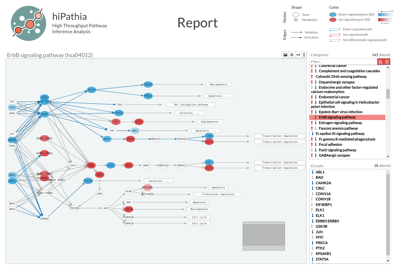
Pathway viewer for differential signaling
Finally, for those users with experience in R, the differential signaling results can be visualized using the hiPathia R package, by subsetting the table to the comparison of interest and using the create_report() function. Here you can find an example of the rich visualization generated by the package: